Free Statistics
of Irreproducible Research!
Description of Statistical Computation | |||||||||||||||||||||||||||||||||||||||||||||||||||||||||||||||||||||||||||||||||||||||||||||||||||||
|---|---|---|---|---|---|---|---|---|---|---|---|---|---|---|---|---|---|---|---|---|---|---|---|---|---|---|---|---|---|---|---|---|---|---|---|---|---|---|---|---|---|---|---|---|---|---|---|---|---|---|---|---|---|---|---|---|---|---|---|---|---|---|---|---|---|---|---|---|---|---|---|---|---|---|---|---|---|---|---|---|---|---|---|---|---|---|---|---|---|---|---|---|---|---|---|---|---|---|---|---|---|
| Author's title | |||||||||||||||||||||||||||||||||||||||||||||||||||||||||||||||||||||||||||||||||||||||||||||||||||||
| Author | *Unverified author* | ||||||||||||||||||||||||||||||||||||||||||||||||||||||||||||||||||||||||||||||||||||||||||||||||||||
| R Software Module | rwasp_notchedbox1.wasp | ||||||||||||||||||||||||||||||||||||||||||||||||||||||||||||||||||||||||||||||||||||||||||||||||||||
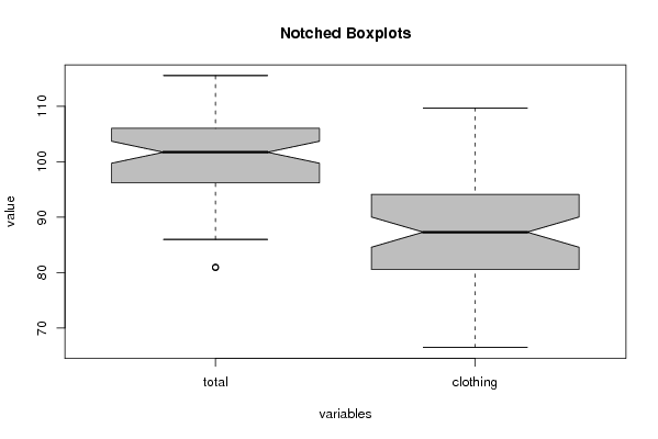
| Title produced by software | Notched Boxplots | ||||||||||||||||||||||||||||||||||||||||||||||||||||||||||||||||||||||||||||||||||||||||||||||||||||
| Date of computation | Fri, 26 Oct 2007 06:31:48 -0700 | ||||||||||||||||||||||||||||||||||||||||||||||||||||||||||||||||||||||||||||||||||||||||||||||||||||
| Cite this page as follows | Statistical Computations at FreeStatistics.org, Office for Research Development and Education, URL https://freestatistics.org/blog/index.php?v=date/2007/Oct/26/e3gf4m47miu91211193405177.htm/, Retrieved Sun, 28 Apr 2024 23:39:05 +0000 | ||||||||||||||||||||||||||||||||||||||||||||||||||||||||||||||||||||||||||||||||||||||||||||||||||||
| Statistical Computations at FreeStatistics.org, Office for Research Development and Education, URL https://freestatistics.org/blog/index.php?pk=1838, Retrieved Sun, 28 Apr 2024 23:39:05 +0000 | |||||||||||||||||||||||||||||||||||||||||||||||||||||||||||||||||||||||||||||||||||||||||||||||||||||
| QR Codes: | |||||||||||||||||||||||||||||||||||||||||||||||||||||||||||||||||||||||||||||||||||||||||||||||||||||
|
| |||||||||||||||||||||||||||||||||||||||||||||||||||||||||||||||||||||||||||||||||||||||||||||||||||||
| Original text written by user: | |||||||||||||||||||||||||||||||||||||||||||||||||||||||||||||||||||||||||||||||||||||||||||||||||||||
| IsPrivate? | No (this computation is public) | ||||||||||||||||||||||||||||||||||||||||||||||||||||||||||||||||||||||||||||||||||||||||||||||||||||
| User-defined keywords | notched boxplot | ||||||||||||||||||||||||||||||||||||||||||||||||||||||||||||||||||||||||||||||||||||||||||||||||||||
| Estimated Impact | 666 | ||||||||||||||||||||||||||||||||||||||||||||||||||||||||||||||||||||||||||||||||||||||||||||||||||||
Tree of Dependent Computations | |||||||||||||||||||||||||||||||||||||||||||||||||||||||||||||||||||||||||||||||||||||||||||||||||||||
| Family? (F = Feedback message, R = changed R code, M = changed R Module, P = changed Parameters, D = changed Data) | |||||||||||||||||||||||||||||||||||||||||||||||||||||||||||||||||||||||||||||||||||||||||||||||||||||
| F [Notched Boxplots] [workshop 3] [2007-10-26 13:31:48] [d06427f3e67cec1f6334fc93f511b0b4] [Current] - RMPD [Mean Plot] [Boxplots Dollar ] [2008-01-14 19:32:01] [74be16979710d4c4e7c6647856088456] - RMPD [Box-Cox Linearity Plot] [Box Cox linearity...] [2008-01-14 22:00:56] [74be16979710d4c4e7c6647856088456] - RMPD [Bivariate Kernel Density Estimation] [Bivariate Kernel ...] [2008-01-14 22:14:00] [74be16979710d4c4e7c6647856088456] - R D [Notched Boxplots] [Q1] [2008-10-28 14:07:27] [c5a66f1c8528a963efc2b82a8519f117] - [Notched Boxplots] [Q1] [2008-11-04 17:45:45] [b1bd16d1f47bfe13feacf1c27a0abba5] - R D [Notched Boxplots] [Q1] [2008-10-28 14:07:27] [3d2d096cc21c6f80db3dd7b8e12effce] - R D [Notched Boxplots] [Wokshop 1, Q1 (Ba2)] [2008-11-06 12:03:44] [488d9a19d3c63b747ac6ad96017e55c8] - RM D [Mean Plot] [Workshop 1, Q2 (Ba2)] [2008-11-06 12:23:47] [488d9a19d3c63b747ac6ad96017e55c8] - RM D [Blocked Bootstrap Plot - Central Tendency] [Workshop 1, Q4 (Ba2)] [2008-11-06 13:03:43] [488d9a19d3c63b747ac6ad96017e55c8] F [Blocked Bootstrap Plot - Central Tendency] [] [2008-11-06 19:21:47] [072bb89749ef40809573ea0372b43d78] - D [Notched Boxplots] [Workshop 1, task ...] [2008-11-06 13:51:03] [488d9a19d3c63b747ac6ad96017e55c8] - D [Notched Boxplots] [] [2008-11-06 14:13:07] [488d9a19d3c63b747ac6ad96017e55c8] - D [Notched Boxplots] [] [2008-11-06 14:19:50] [488d9a19d3c63b747ac6ad96017e55c8] - D [Notched Boxplots] [] [2008-11-06 14:22:51] [488d9a19d3c63b747ac6ad96017e55c8] - D [Notched Boxplots] [] [2008-11-06 14:27:04] [488d9a19d3c63b747ac6ad96017e55c8] - D [Notched Boxplots] [Workshop 1, task ...] [2008-11-06 14:39:39] [488d9a19d3c63b747ac6ad96017e55c8] F RM D [Kendall tau Correlation Matrix] [] [2008-11-06 17:09:26] [488d9a19d3c63b747ac6ad96017e55c8] - R D [Notched Boxplots] [Q1] [2008-10-28 14:16:45] [c5a66f1c8528a963efc2b82a8519f117] F D [Notched Boxplots] [Q1: test the hypo...] [2008-10-28 20:21:27] [1e1d8320a8a1170c475bf6e4ce119de6] F D [Notched Boxplots] [Q3 A financial co...] [2008-11-01 12:21:14] [1e1d8320a8a1170c475bf6e4ce119de6] F D [Notched Boxplots] [Task 2: reuse the...] [2008-10-28 20:52:58] [1e1d8320a8a1170c475bf6e4ce119de6] F [Notched Boxplots] [] [2008-11-06 19:25:19] [072bb89749ef40809573ea0372b43d78] F D [Notched Boxplots] [Herproducering ta...] [2008-10-29 11:37:57] [819b576fab25b35cfda70f80599828ec] - D [Notched Boxplots] [reproduce Q1] [2008-10-29 11:45:56] [d2d412c7f4d35ffbf5ee5ee89db327d4] F D [Notched Boxplots] [Nothched boxplots...] [2008-10-29 11:39:06] [b635de6fc42b001d22cbe6e730fec936] F D [Notched Boxplots] [Taak 1, Q1] [2008-10-29 15:50:25] [deb3c14ac9e4607a6d84fc9d0e0e6cc2] F D [Notched Boxplots] [Q1 notched boxplot] [2008-10-30 08:45:36] [fe7291e888d31b8c4db0b24d6c0f75c6] F D [Notched Boxplots] [Hypothesis Testin...] [2008-10-29 11:51:48] [063e4b67ad7d3a8a83eccec794cd5aa7] - [Notched Boxplots] [Hypothesis Testin...] [2008-10-29 12:20:11] [063e4b67ad7d3a8a83eccec794cd5aa7] F R [Notched Boxplots] [Hypothesis Testin...] [2008-10-29 12:33:08] [063e4b67ad7d3a8a83eccec794cd5aa7] - D [Notched Boxplots] [hypothesis testin...] [2008-10-29 11:51:25] [a18c43c8b63fa6800a53bb187b9ddd45] F D [Notched Boxplots] [hypothesis testin...] [2008-10-29 11:51:25] [631938996a408f8d8cf3d9850ca0cd03] F R [Notched Boxplots] [hypothesis testin...] [2008-10-29 12:19:42] [631938996a408f8d8cf3d9850ca0cd03] F D [Notched Boxplots] [Q1 notched boxplot] [2008-10-29 13:04:27] [7173087adebe3e3a714c80ea2417b3eb] F R PD [Notched Boxplots] [taak 2 notched bo...] [2008-10-29 14:38:58] [7173087adebe3e3a714c80ea2417b3eb] F R [Notched Boxplots] [Task 3 notched bo...] [2008-10-29 14:51:53] [7173087adebe3e3a714c80ea2417b3eb] F P [Notched Boxplots] [task 3 ] [2008-11-03 17:22:27] [e43247bc0ab243a5af99ac7f55ba0b41] F P [Notched Boxplots] [task 2] [2008-11-03 17:21:02] [e43247bc0ab243a5af99ac7f55ba0b41] - RMPD [Star Plot] [Starplot: Auto ca...] [2008-11-11 23:56:07] [944cfe91fab3d898afdbc7f6b8914047] F [Notched Boxplots] [q1] [2008-11-03 17:13:13] [e43247bc0ab243a5af99ac7f55ba0b41] F R D [Notched Boxplots] [] [2008-10-29 13:33:23] [8e4e5f204c24e6d05647858dae308d17] - D [Notched Boxplots] [Mediaan kledij < ...] [2008-10-29 13:49:59] [495cd80c1a9baafb03c09cd9ab8d8fb5] F D [Notched Boxplots] [Mediaan kledij < ...] [2008-10-29 13:57:22] [495cd80c1a9baafb03c09cd9ab8d8fb5] F PD [Notched Boxplots] [Mediaan afzetprij...] [2008-10-29 15:39:02] [495cd80c1a9baafb03c09cd9ab8d8fb5] F PD [Notched Boxplots] [Mediaan investeri...] [2008-10-29 15:49:49] [495cd80c1a9baafb03c09cd9ab8d8fb5] F D [Notched Boxplots] [Logaritmen mediaa...] [2008-10-29 16:49:14] [495cd80c1a9baafb03c09cd9ab8d8fb5] F R D [Notched Boxplots] [Notched Boxplots] [2008-10-29 16:25:40] [b518240a1c80d4f939bf8b3e34f77cec] - R [Notched Boxplots] [Q3] [2008-10-29 17:55:00] [b518240a1c80d4f939bf8b3e34f77cec] [Truncated] | |||||||||||||||||||||||||||||||||||||||||||||||||||||||||||||||||||||||||||||||||||||||||||||||||||||
| Feedback Forum | |||||||||||||||||||||||||||||||||||||||||||||||||||||||||||||||||||||||||||||||||||||||||||||||||||||
Post a new message | |||||||||||||||||||||||||||||||||||||||||||||||||||||||||||||||||||||||||||||||||||||||||||||||||||||
Dataset | |||||||||||||||||||||||||||||||||||||||||||||||||||||||||||||||||||||||||||||||||||||||||||||||||||||
| Dataseries X: | |||||||||||||||||||||||||||||||||||||||||||||||||||||||||||||||||||||||||||||||||||||||||||||||||||||
110,40 109,20 96,40 88,60 101,90 94,30 106,20 98,30 81,00 86,40 94,70 80,60 101,00 104,10 109,40 108,20 102,30 93,40 90,70 71,90 96,20 94,10 96,10 94,90 106,00 96,40 103,10 91,10 102,00 84,40 104,70 86,40 86,00 88,00 92,10 75,10 106,90 109,70 112,60 103,00 101,70 82,10 92,00 68,00 97,40 96,40 97,00 94,30 105,40 90,00 102,70 88,00 98,10 76,10 104,50 82,50 87,40 81,40 89,90 66,50 109,80 97,20 111,70 94,10 98,60 80,70 96,90 70,50 95,10 87,80 97,00 89,50 112,70 99,60 102,90 84,20 97,40 75,10 111,40 92,00 87,40 80,80 96,80 73,10 114,10 99,80 110,30 90,00 103,90 83,10 101,60 72,40 94,60 78,80 95,90 87,30 104,70 91,00 102,80 80,10 98,10 73,60 113,90 86,40 80,90 74,50 95,70 71,20 113,20 92,40 105,90 81,50 108,80 85,30 102,30 69,90 99,00 84,20 100,70 90,70 115,50 100,30 | |||||||||||||||||||||||||||||||||||||||||||||||||||||||||||||||||||||||||||||||||||||||||||||||||||||
Tables (Output of Computation) | |||||||||||||||||||||||||||||||||||||||||||||||||||||||||||||||||||||||||||||||||||||||||||||||||||||
| |||||||||||||||||||||||||||||||||||||||||||||||||||||||||||||||||||||||||||||||||||||||||||||||||||||
Figures (Output of Computation) | |||||||||||||||||||||||||||||||||||||||||||||||||||||||||||||||||||||||||||||||||||||||||||||||||||||
Input Parameters & R Code | |||||||||||||||||||||||||||||||||||||||||||||||||||||||||||||||||||||||||||||||||||||||||||||||||||||
| Parameters (Session): | |||||||||||||||||||||||||||||||||||||||||||||||||||||||||||||||||||||||||||||||||||||||||||||||||||||
| par1 = grey ; | |||||||||||||||||||||||||||||||||||||||||||||||||||||||||||||||||||||||||||||||||||||||||||||||||||||
| Parameters (R input): | |||||||||||||||||||||||||||||||||||||||||||||||||||||||||||||||||||||||||||||||||||||||||||||||||||||
| par1 = grey ; | |||||||||||||||||||||||||||||||||||||||||||||||||||||||||||||||||||||||||||||||||||||||||||||||||||||
| R code (references can be found in the software module): | |||||||||||||||||||||||||||||||||||||||||||||||||||||||||||||||||||||||||||||||||||||||||||||||||||||
z <- as.data.frame(t(y)) | |||||||||||||||||||||||||||||||||||||||||||||||||||||||||||||||||||||||||||||||||||||||||||||||||||||