Free Statistics
of Irreproducible Research!
Description of Statistical Computation | ||||||||||||||||||||||||||||||||||||
|---|---|---|---|---|---|---|---|---|---|---|---|---|---|---|---|---|---|---|---|---|---|---|---|---|---|---|---|---|---|---|---|---|---|---|---|---|
| Author's title | ||||||||||||||||||||||||||||||||||||
| Author | *Unverified author* | |||||||||||||||||||||||||||||||||||
| R Software Module | rwasp_backtobackhist.wasp | |||||||||||||||||||||||||||||||||||
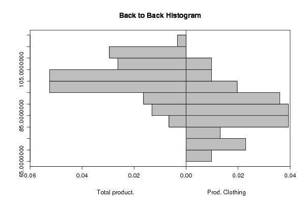
| Title produced by software | Back to Back Histogram | |||||||||||||||||||||||||||||||||||
| Date of computation | Thu, 18 Oct 2007 03:14:23 -0700 | |||||||||||||||||||||||||||||||||||
| Cite this page as follows | Statistical Computations at FreeStatistics.org, Office for Research Development and Education, URL https://freestatistics.org/blog/index.php?v=date/2007/Oct/18/t7cauiw7lrza8kp1192702308.htm/, Retrieved Sun, 28 Apr 2024 23:08:06 +0000 | |||||||||||||||||||||||||||||||||||
| Statistical Computations at FreeStatistics.org, Office for Research Development and Education, URL https://freestatistics.org/blog/index.php?pk=978, Retrieved Sun, 28 Apr 2024 23:08:06 +0000 | ||||||||||||||||||||||||||||||||||||
| QR Codes: | ||||||||||||||||||||||||||||||||||||
|
| ||||||||||||||||||||||||||||||||||||
| Original text written by user: | ||||||||||||||||||||||||||||||||||||
| IsPrivate? | No (this computation is public) | |||||||||||||||||||||||||||||||||||
| User-defined keywords | Q2 | |||||||||||||||||||||||||||||||||||
| Estimated Impact | 469 | |||||||||||||||||||||||||||||||||||
Tree of Dependent Computations | ||||||||||||||||||||||||||||||||||||
| Family? (F = Feedback message, R = changed R code, M = changed R Module, P = changed Parameters, D = changed Data) | ||||||||||||||||||||||||||||||||||||
| F [Back to Back Histogram] [Q2 Total / Clothi...] [2007-10-18 10:14:23] [1a83104d28786df2e24859e2e02dc234] [Current] F PD [Back to Back Histogram] [Q2 - Comparison o...] [2008-10-15 17:35:53] [a57f5cc542637534b8bb5bcb4d37eab1] - PD [Back to Back Histogram] [investigating ass...] [2008-10-16 22:39:41] [cbd3d88cd5aad6543e769146e7e26b0c] - RMPD [Kendall tau Rank Correlation] [Kendall Tau Corre...] [2008-12-18 11:07:47] [b591abfa820a394aeb0c5ebd9cfa1091] - RMPD [Kendall tau Rank Correlation] [Kendall Tau Corre...] [2008-12-18 11:22:42] [b591abfa820a394aeb0c5ebd9cfa1091] - RMPD [Kendall tau Rank Correlation] [Kendall Tau Corre...] [2008-12-18 11:28:10] [b591abfa820a394aeb0c5ebd9cfa1091] - PD [Back to Back Histogram] [B2B histogram Tot...] [2008-10-17 11:32:20] [1e1d8320a8a1170c475bf6e4ce119de6] - R PD [Back to Back Histogram] [total production ...] [2008-10-18 11:02:44] [529a65e524c481ca1098665a9566b89f] - PD [Back to Back Histogram] [Back-to-back hist...] [2008-10-19 15:32:37] [5e74953d94072114d25d7276793b561e] - R P [Back to Back Histogram] [total production ...] [2008-10-18 11:06:28] [529a65e524c481ca1098665a9566b89f] - R D [Back to Back Histogram] [Total prod vs pro...] [2008-10-17 11:47:11] [3d2d096cc21c6f80db3dd7b8e12effce] F D [Back to Back Histogram] [back to back hist...] [2008-10-17 14:28:24] [cf45c678b7899ee33d7b061948f80651] F D [Back to Back Histogram] [Histogram] [2008-10-17 21:01:48] [8b0d202c3a0c4ea223fd8b8e731dacd8] - PD [Back to Back Histogram] [B2B histogram tot...] [2008-10-18 13:16:34] [d32f94eec6fe2d8c421bd223368a5ced] - RM D [Pearson Correlation] [Pearson correlati...] [2008-10-18 15:58:27] [b943bd7078334192ff8343563ee31113] F D [Back to Back Histogram] [Back-to-back hist...] [2008-10-19 08:27:00] [4396f984ebeab43316cd6baa88a4fd40] F D [Back to Back Histogram] [Investigating Ass...] [2008-10-19 08:58:58] [6743688719638b0cb1c0a6e0bf433315] F D [Back to Back Histogram] [Task 1 - Q2 - Bac...] [2008-10-19 10:43:59] [33f4701c7363e8b81858dafbf0350eed] F [Back to Back Histogram] [investigating ass Q2] [2008-10-20 23:01:21] [b641c14ac36cb6fee377f3b099dcac19] - PD [Back to Back Histogram] [Q2 totale product...] [2008-10-19 11:49:19] [e5d91604aae608e98a8ea24759233f66] F D [Back to Back Histogram] [Task 1 Q2] [2008-10-19 12:38:14] [86761fc994bdf34e4f4ab5b8e1d9e1c3] - D [Back to Back Histogram] [] [2008-10-19 15:54:42] [8d78428855b119373cac369316c08983] F D [Back to Back Histogram] [] [2008-10-19 16:11:12] [8d78428855b119373cac369316c08983] F PD [Back to Back Histogram] [Q2 Distributions ...] [2008-10-19 17:01:36] [cf9c64468d04c2c4dd548cc66b4e3677] F PD [Back to Back Histogram] [Q2 Back to Back h...] [2008-10-20 08:58:32] [38f43994ada0e6172896e12525dcc585] - R D [Back to Back Histogram] [Q2 Back To Back] [2008-10-20 11:49:44] [74be16979710d4c4e7c6647856088456] F D [Back to Back Histogram] [q2 b2b] [2008-10-20 12:01:26] [dd679c9a7f849ed0333823e9c020c5a6] F D [Back to Back Histogram] [Histogram: Totale...] [2008-10-20 12:52:54] [1d988b04e8982749ec309eda662241b4] F R D [Back to Back Histogram] [Histogram: Totale...] [2008-10-20 12:55:08] [a7f04e0e73ce3683561193958d653479] F PD [Back to Back Histogram] [Totale Productie ...] [2008-10-20 13:29:40] [1376d48f59a7212e8dd85a587491a69b] F D [Back to Back Histogram] [Back to back tota...] [2008-10-20 13:40:48] [e562c84ebfc887cc5a7a99782625ca3b] F D [Back to Back Histogram] [Workshop 2] [2008-10-20 13:53:46] [b990da0cb3aa26f81c0c422f8ba66d53] - PD [Back to Back Histogram] [Distributions of ...] [2008-10-20 13:54:23] [43d870b30ac8a7afeb5de9ee11dcfc1a] F R D [Back to Back Histogram] [Q2 is de totale d...] [2008-10-20 14:25:15] [84dda5145c389bd11bcc662bd33fe4ba] F D [Back to Back Histogram] [Q2: Distributie] [2008-10-20 15:14:50] [82d201ca7b4e7cd2c6f885d29b5b6937] F R D [Back to Back Histogram] [ taak 1 vraag 2 K...] [2008-10-20 15:18:41] [f21e40d80585aedc38277df87deba3c6] F [Back to Back Histogram] [back-to-back hist...] [2008-10-20 17:27:34] [e242ef2117cdd06cb7827a9ae01189a0] F D [Back to Back Histogram] [Q2 Back-to-back h...] [2008-10-20 16:11:06] [2d4aec5ed1856c4828162be37be304d9] F D [Back to Back Histogram] [back to back hist...] [2008-10-20 16:12:34] [fe7291e888d31b8c4db0b24d6c0f75c6] F [Back to Back Histogram] [Back to back hist...] [2008-10-20 16:53:09] [b635de6fc42b001d22cbe6e730fec936] - RMPD [Pearson Correlation] [Verbetering Q6] [2008-10-21 15:52:34] [2a0ad3a9bcadca2da0acb91636601c6c] - RMPD [Pearson Correlation] [Verbetering Q6] [2008-10-21 15:52:34] [2a0ad3a9bcadca2da0acb91636601c6c] - RMPD [Pearson Correlation] [Verbetering Q4] [2008-10-21 15:52:34] [2a0ad3a9bcadca2da0acb91636601c6c] - PD [Back to Back Histogram] [back to back] [2008-12-18 15:16:15] [fe7291e888d31b8c4db0b24d6c0f75c6] - PD [Back to Back Histogram] [back to back] [2008-12-18 15:58:12] [fe7291e888d31b8c4db0b24d6c0f75c6] - PD [Back to Back Histogram] [back to back] [2008-12-18 16:00:12] [fe7291e888d31b8c4db0b24d6c0f75c6] - P [Back to Back Histogram] [back to back] [2008-12-18 21:40:03] [fe7291e888d31b8c4db0b24d6c0f75c6] - D [Back to Back Histogram] [1] [2008-12-22 18:23:53] [fe7291e888d31b8c4db0b24d6c0f75c6] - PD [Back to Back Histogram] [back to back] [2008-12-18 15:21:08] [fe7291e888d31b8c4db0b24d6c0f75c6] [Truncated] | ||||||||||||||||||||||||||||||||||||
| Feedback Forum | ||||||||||||||||||||||||||||||||||||
Post a new message | ||||||||||||||||||||||||||||||||||||
Dataset | ||||||||||||||||||||||||||||||||||||
| Dataseries X: | ||||||||||||||||||||||||||||||||||||
110.40 96.40 101.90 106.20 81.00 94.70 101.00 109.40 102.30 90.70 96.20 96.10 106.00 103.10 102.00 104.70 86.00 92.10 106.90 112.60 101.70 92.00 97.40 97.00 105.40 102.70 98.10 104.50 87.40 89.90 109.80 111.70 98.60 96.90 95.10 97.00 112.70 102.90 97.40 111.40 87.40 96.80 114.10 110.30 103.90 101.60 94.60 95.90 104.70 102.80 98.10 113.90 80.90 95.70 113.20 105.90 108.80 102.30 99.00 100.70 115.50 | ||||||||||||||||||||||||||||||||||||
| Dataseries Y: | ||||||||||||||||||||||||||||||||||||
109.20 88.60 94.30 98.30 86.40 80.60 104.10 108.20 93.40 71.90 94.10 94.90 96.40 91.10 84.40 86.40 88.00 75.10 109.70 103.00 82.10 68.00 96.40 94.30 90.00 88.00 76.10 82.50 81.40 66.50 97.20 94.10 80.70 70.50 87.80 89.50 99.60 84.20 75.10 92.00 80.80 73.10 99.80 90.00 83.10 72.40 78.80 87.30 91.00 80.10 73.60 86.40 74.50 71.20 92.40 81.50 85.30 69.90 84.20 90.70 100.30 | ||||||||||||||||||||||||||||||||||||
Tables (Output of Computation) | ||||||||||||||||||||||||||||||||||||
| ||||||||||||||||||||||||||||||||||||
Figures (Output of Computation) | ||||||||||||||||||||||||||||||||||||
Input Parameters & R Code | ||||||||||||||||||||||||||||||||||||
| Parameters (Session): | ||||||||||||||||||||||||||||||||||||
| par1 = grey ; par2 = grey ; par3 = TRUE ; par4 = Total product. ; par5 = Prod. Clothing ; | ||||||||||||||||||||||||||||||||||||
| Parameters (R input): | ||||||||||||||||||||||||||||||||||||
| par1 = grey ; par2 = grey ; par3 = TRUE ; par4 = Total product. ; par5 = Prod. Clothing ; | ||||||||||||||||||||||||||||||||||||
| R code (references can be found in the software module): | ||||||||||||||||||||||||||||||||||||
if (par3 == 'TRUE') par3 <- TRUE | ||||||||||||||||||||||||||||||||||||