Repository of Reproducible Computations

Free Statistics

of Irreproducible Research!

Author's title

Author

*Unverified author*

R Software Module

rwasp_autocorrelation.wasp

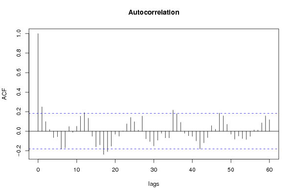
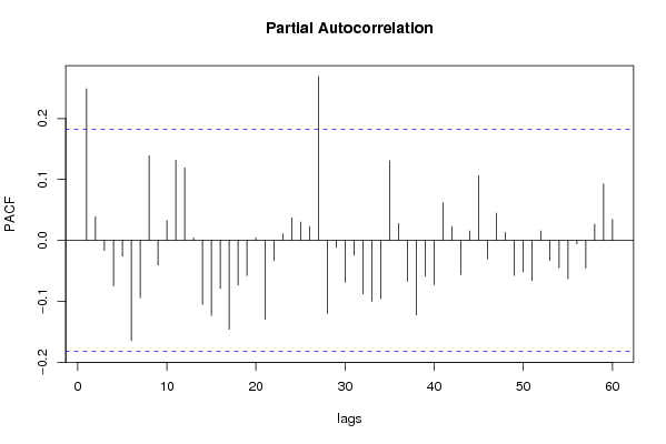
Title produced by software

(Partial) Autocorrelation Function

Date of computation

Mon, 03 Dec 2007 04:20:48 -0700

Cite this page as follows

Statistical Computations at FreeStatistics.org, Office for Research Development and Education, URL https://freestatistics.org/blog/index.php?v=date/2007/Dec/03/t1196680157s7ajl5lmyhi7xgj.htm/, Retrieved Fri, 03 May 2024 16:19:33 +0000

Statistical Computations at FreeStatistics.org, Office for Research Development and Education, URL https://freestatistics.org/blog/index.php?pk=2319, Retrieved Fri, 03 May 2024 16:19:33 +0000

QR Codes:

Paste this QR Code to cite your computation.

Original text written by user:

IsPrivate?

No (this computation is public)

User-defined keywords

ex012008

Estimated Impact

590

Family? (F = Feedback message, R = changed R code, M = changed R Module, P = changed Parameters, D = changed Data)

-       [(Partial) Autocorrelation Function] [omzet] [2007-12-03 11:20:48] [ef257666c09b3678397177defae7fd99] [Current]
- RMPD    [Univariate Explorative Data Analysis] [paper:investeringen] [2008-01-02 15:28:12] [30a905e6cad0f132038c9ca2894b4669] 
F   PD    [(Partial) Autocorrelation Function] [Various EDA topic...] [2008-11-12 10:44:14] [c29178f7f550574a75dc881e636e0923] 
F RMPD      [Trivariate Scatterplots] [Various EDA topic...] [2008-11-12 11:00:11] [c29178f7f550574a75dc881e636e0923] 
- RMP         [Partial Correlation] [Q1 partial correl...] [2008-11-15 13:11:00] [ed2ba3b6182103c15c0ab511ae4e6284] 
F RMPD      [Hierarchical Clustering] [hierarchial clust...] [2008-11-12 11:21:49] [c29178f7f550574a75dc881e636e0923] 
F RMPD      [Box-Cox Linearity Plot] [Various topics ab...] [2008-11-12 11:30:21] [c29178f7f550574a75dc881e636e0923] 

Feedback Forum

Post a new message

Dataseries X:

Download CSV

Histogram

Boxplots

Summary of compuational transaction
Raw Input	view raw input (R code)
Raw Output	view raw output of R engine
Computing time	2 seconds
R Server	'Herman Ole Andreas Wold' @ 193.190.124.10:1001

\begin{tabular}{lllllllll}
\hline
Summary of compuational transaction \tabularnewline
Raw Input & view raw input (R code)  \tabularnewline
Raw Output & view raw output of R engine  \tabularnewline
Computing time & 2 seconds \tabularnewline
R Server & 'Herman Ole Andreas Wold' @ 193.190.124.10:1001 \tabularnewline
\hline
\end{tabular}
%Source: https://freestatistics.org/blog/index.php?pk=2319&T=0

[TABLE]
[ROW][C]Summary of compuational transaction[/C][/ROW]
[ROW][C]Raw Input[/C][C]view raw input (R code) [/C][/ROW]
[ROW][C]Raw Output[/C][C]view raw output of R engine [/C][/ROW]
[ROW][C]Computing time[/C][C]2 seconds[/C][/ROW]
[ROW][C]R Server[/C][C]'Herman Ole Andreas Wold' @ 193.190.124.10:1001[/C][/ROW]
[/TABLE]
Source: https://freestatistics.org/blog/index.php?pk=2319&T=0

Globally Unique Identifier (entire table): ba.freestatistics.org/blog/index.php?pk=2319&T=0

As an alternative you can also use a QR Code:

The GUIDs for individual cells are displayed in the table below:

Summary of compuational transaction
Raw Input	view raw input (R code)
Raw Output	view raw output of R engine
Computing time	2 seconds
R Server	'Herman Ole Andreas Wold' @ 193.190.124.10:1001

Autocorrelation Function
Time lag k	ACF(k)	T-STAT	P-value
0	1	10.7703	0
1	0.248937	2.6811	0.004203
2	0.098582	1.0618	0.145275
3	0.017833	0.1921	0.424015
4	-0.065099	-0.7011	0.757688
5	-0.057077	-0.6147	0.730032
6	-0.182043	-1.9607	0.973842
7	-0.170193	-1.833	0.965319
8	0.048047	0.5175	0.302902
9	-0.011478	-0.1236	0.549087
10	0.050928	0.5485	0.292199
11	0.154412	1.6631	0.049499
12	0.190374	2.0504	0.02129
13	0.133115	1.4337	0.077176
14	-0.052059	-0.5607	0.711957
15	-0.160447	-1.7281	0.956682
16	-0.140289	-1.511	0.933241
17	-0.237442	-2.5573	0.994081
18	-0.209334	-2.2546	0.986982
19	-0.154154	-1.6603	0.950221
20	-0.030775	-0.3315	0.629552
21	-0.051018	-0.5495	0.708132
22	0.003081	0.0332	0.486792
23	0.075645	0.8147	0.20845
24	0.141643	1.5255	0.064923
25	0.097077	1.0455	0.148972
26	0.011106	0.1196	0.452497
27	0.155258	1.6722	0.048592
28	-0.07802	-0.8403	0.798765
29	-0.105886	-1.1404	0.871771
30	-0.150572	-1.6217	0.94621
31	-0.092841	-0.9999	0.840288
32	-0.021263	-0.229	0.590368
33	-0.067554	-0.7276	0.76583
34	-0.068048	-0.7329	0.76745
35	0.216243	2.329	0.010795
36	0.17897	1.9276	0.028177
37	0.090922	0.9793	0.164743
38	-0.021673	-0.2334	0.592078
39	-0.046764	-0.5037	0.692274
40	-0.053237	-0.5734	0.71625
41	-0.099438	-1.071	0.856798
42	-0.181632	-1.9562	0.97358
43	-0.118737	-1.2788	0.898246
44	-0.065122	-0.7014	0.757767
45	0.056381	0.6072	0.272439
46	0.020256	0.2182	0.413844
47	0.185348	1.9963	0.024124
48	0.157527	1.6966	0.046225
49	0.069974	0.7536	0.226294
50	-0.030439	-0.3278	0.628187
51	-0.081456	-0.8773	0.808933
52	-0.049058	-0.5284	0.700875
53	-0.075072	-0.8085	0.789785
54	-0.084867	-0.914	0.818707
55	-0.052563	-0.5661	0.713798
56	0.012593	0.1356	0.446172
57	0.011644	0.1254	0.450207
58	0.085659	0.9226	0.179072
59	0.157257	1.6937	0.046502

\begin{tabular}{lllllllll}
\hline
Autocorrelation Function \tabularnewline
Time lag k & ACF(k) & T-STAT & P-value \tabularnewline
0 & 1 & 10.7703 & 0 \tabularnewline
1 & 0.248937 & 2.6811 & 0.004203 \tabularnewline
2 & 0.098582 & 1.0618 & 0.145275 \tabularnewline
3 & 0.017833 & 0.1921 & 0.424015 \tabularnewline
4 & -0.065099 & -0.7011 & 0.757688 \tabularnewline
5 & -0.057077 & -0.6147 & 0.730032 \tabularnewline
6 & -0.182043 & -1.9607 & 0.973842 \tabularnewline
7 & -0.170193 & -1.833 & 0.965319 \tabularnewline
8 & 0.048047 & 0.5175 & 0.302902 \tabularnewline
9 & -0.011478 & -0.1236 & 0.549087 \tabularnewline
10 & 0.050928 & 0.5485 & 0.292199 \tabularnewline
11 & 0.154412 & 1.6631 & 0.049499 \tabularnewline
12 & 0.190374 & 2.0504 & 0.02129 \tabularnewline
13 & 0.133115 & 1.4337 & 0.077176 \tabularnewline
14 & -0.052059 & -0.5607 & 0.711957 \tabularnewline
15 & -0.160447 & -1.7281 & 0.956682 \tabularnewline
16 & -0.140289 & -1.511 & 0.933241 \tabularnewline
17 & -0.237442 & -2.5573 & 0.994081 \tabularnewline
18 & -0.209334 & -2.2546 & 0.986982 \tabularnewline
19 & -0.154154 & -1.6603 & 0.950221 \tabularnewline
20 & -0.030775 & -0.3315 & 0.629552 \tabularnewline
21 & -0.051018 & -0.5495 & 0.708132 \tabularnewline
22 & 0.003081 & 0.0332 & 0.486792 \tabularnewline
23 & 0.075645 & 0.8147 & 0.20845 \tabularnewline
24 & 0.141643 & 1.5255 & 0.064923 \tabularnewline
25 & 0.097077 & 1.0455 & 0.148972 \tabularnewline
26 & 0.011106 & 0.1196 & 0.452497 \tabularnewline
27 & 0.155258 & 1.6722 & 0.048592 \tabularnewline
28 & -0.07802 & -0.8403 & 0.798765 \tabularnewline
29 & -0.105886 & -1.1404 & 0.871771 \tabularnewline
30 & -0.150572 & -1.6217 & 0.94621 \tabularnewline
31 & -0.092841 & -0.9999 & 0.840288 \tabularnewline
32 & -0.021263 & -0.229 & 0.590368 \tabularnewline
33 & -0.067554 & -0.7276 & 0.76583 \tabularnewline
34 & -0.068048 & -0.7329 & 0.76745 \tabularnewline
35 & 0.216243 & 2.329 & 0.010795 \tabularnewline
36 & 0.17897 & 1.9276 & 0.028177 \tabularnewline
37 & 0.090922 & 0.9793 & 0.164743 \tabularnewline
38 & -0.021673 & -0.2334 & 0.592078 \tabularnewline
39 & -0.046764 & -0.5037 & 0.692274 \tabularnewline
40 & -0.053237 & -0.5734 & 0.71625 \tabularnewline
41 & -0.099438 & -1.071 & 0.856798 \tabularnewline
42 & -0.181632 & -1.9562 & 0.97358 \tabularnewline
43 & -0.118737 & -1.2788 & 0.898246 \tabularnewline
44 & -0.065122 & -0.7014 & 0.757767 \tabularnewline
45 & 0.056381 & 0.6072 & 0.272439 \tabularnewline
46 & 0.020256 & 0.2182 & 0.413844 \tabularnewline
47 & 0.185348 & 1.9963 & 0.024124 \tabularnewline
48 & 0.157527 & 1.6966 & 0.046225 \tabularnewline
49 & 0.069974 & 0.7536 & 0.226294 \tabularnewline
50 & -0.030439 & -0.3278 & 0.628187 \tabularnewline
51 & -0.081456 & -0.8773 & 0.808933 \tabularnewline
52 & -0.049058 & -0.5284 & 0.700875 \tabularnewline
53 & -0.075072 & -0.8085 & 0.789785 \tabularnewline
54 & -0.084867 & -0.914 & 0.818707 \tabularnewline
55 & -0.052563 & -0.5661 & 0.713798 \tabularnewline
56 & 0.012593 & 0.1356 & 0.446172 \tabularnewline
57 & 0.011644 & 0.1254 & 0.450207 \tabularnewline
58 & 0.085659 & 0.9226 & 0.179072 \tabularnewline
59 & 0.157257 & 1.6937 & 0.046502 \tabularnewline
\hline
\end{tabular}
%Source: https://freestatistics.org/blog/index.php?pk=2319&T=1

[TABLE]
[ROW][C]Autocorrelation Function[/C][/ROW]
[ROW][C]Time lag k[/C][C]ACF(k)[/C][C]T-STAT[/C][C]P-value[/C][/ROW]
[ROW][C]0[/C][C]1[/C][C]10.7703[/C][C]0[/C][/ROW]
[ROW][C]1[/C][C]0.248937[/C][C]2.6811[/C][C]0.004203[/C][/ROW]
[ROW][C]2[/C][C]0.098582[/C][C]1.0618[/C][C]0.145275[/C][/ROW]
[ROW][C]3[/C][C]0.017833[/C][C]0.1921[/C][C]0.424015[/C][/ROW]
[ROW][C]4[/C][C]-0.065099[/C][C]-0.7011[/C][C]0.757688[/C][/ROW]
[ROW][C]5[/C][C]-0.057077[/C][C]-0.6147[/C][C]0.730032[/C][/ROW]
[ROW][C]6[/C][C]-0.182043[/C][C]-1.9607[/C][C]0.973842[/C][/ROW]
[ROW][C]7[/C][C]-0.170193[/C][C]-1.833[/C][C]0.965319[/C][/ROW]
[ROW][C]8[/C][C]0.048047[/C][C]0.5175[/C][C]0.302902[/C][/ROW]
[ROW][C]9[/C][C]-0.011478[/C][C]-0.1236[/C][C]0.549087[/C][/ROW]
[ROW][C]10[/C][C]0.050928[/C][C]0.5485[/C][C]0.292199[/C][/ROW]
[ROW][C]11[/C][C]0.154412[/C][C]1.6631[/C][C]0.049499[/C][/ROW]
[ROW][C]12[/C][C]0.190374[/C][C]2.0504[/C][C]0.02129[/C][/ROW]
[ROW][C]13[/C][C]0.133115[/C][C]1.4337[/C][C]0.077176[/C][/ROW]
[ROW][C]14[/C][C]-0.052059[/C][C]-0.5607[/C][C]0.711957[/C][/ROW]
[ROW][C]15[/C][C]-0.160447[/C][C]-1.7281[/C][C]0.956682[/C][/ROW]
[ROW][C]16[/C][C]-0.140289[/C][C]-1.511[/C][C]0.933241[/C][/ROW]
[ROW][C]17[/C][C]-0.237442[/C][C]-2.5573[/C][C]0.994081[/C][/ROW]
[ROW][C]18[/C][C]-0.209334[/C][C]-2.2546[/C][C]0.986982[/C][/ROW]
[ROW][C]19[/C][C]-0.154154[/C][C]-1.6603[/C][C]0.950221[/C][/ROW]
[ROW][C]20[/C][C]-0.030775[/C][C]-0.3315[/C][C]0.629552[/C][/ROW]
[ROW][C]21[/C][C]-0.051018[/C][C]-0.5495[/C][C]0.708132[/C][/ROW]
[ROW][C]22[/C][C]0.003081[/C][C]0.0332[/C][C]0.486792[/C][/ROW]
[ROW][C]23[/C][C]0.075645[/C][C]0.8147[/C][C]0.20845[/C][/ROW]
[ROW][C]24[/C][C]0.141643[/C][C]1.5255[/C][C]0.064923[/C][/ROW]
[ROW][C]25[/C][C]0.097077[/C][C]1.0455[/C][C]0.148972[/C][/ROW]
[ROW][C]26[/C][C]0.011106[/C][C]0.1196[/C][C]0.452497[/C][/ROW]
[ROW][C]27[/C][C]0.155258[/C][C]1.6722[/C][C]0.048592[/C][/ROW]
[ROW][C]28[/C][C]-0.07802[/C][C]-0.8403[/C][C]0.798765[/C][/ROW]
[ROW][C]29[/C][C]-0.105886[/C][C]-1.1404[/C][C]0.871771[/C][/ROW]
[ROW][C]30[/C][C]-0.150572[/C][C]-1.6217[/C][C]0.94621[/C][/ROW]
[ROW][C]31[/C][C]-0.092841[/C][C]-0.9999[/C][C]0.840288[/C][/ROW]
[ROW][C]32[/C][C]-0.021263[/C][C]-0.229[/C][C]0.590368[/C][/ROW]
[ROW][C]33[/C][C]-0.067554[/C][C]-0.7276[/C][C]0.76583[/C][/ROW]
[ROW][C]34[/C][C]-0.068048[/C][C]-0.7329[/C][C]0.76745[/C][/ROW]
[ROW][C]35[/C][C]0.216243[/C][C]2.329[/C][C]0.010795[/C][/ROW]
[ROW][C]36[/C][C]0.17897[/C][C]1.9276[/C][C]0.028177[/C][/ROW]
[ROW][C]37[/C][C]0.090922[/C][C]0.9793[/C][C]0.164743[/C][/ROW]
[ROW][C]38[/C][C]-0.021673[/C][C]-0.2334[/C][C]0.592078[/C][/ROW]
[ROW][C]39[/C][C]-0.046764[/C][C]-0.5037[/C][C]0.692274[/C][/ROW]
[ROW][C]40[/C][C]-0.053237[/C][C]-0.5734[/C][C]0.71625[/C][/ROW]
[ROW][C]41[/C][C]-0.099438[/C][C]-1.071[/C][C]0.856798[/C][/ROW]
[ROW][C]42[/C][C]-0.181632[/C][C]-1.9562[/C][C]0.97358[/C][/ROW]
[ROW][C]43[/C][C]-0.118737[/C][C]-1.2788[/C][C]0.898246[/C][/ROW]
[ROW][C]44[/C][C]-0.065122[/C][C]-0.7014[/C][C]0.757767[/C][/ROW]
[ROW][C]45[/C][C]0.056381[/C][C]0.6072[/C][C]0.272439[/C][/ROW]
[ROW][C]46[/C][C]0.020256[/C][C]0.2182[/C][C]0.413844[/C][/ROW]
[ROW][C]47[/C][C]0.185348[/C][C]1.9963[/C][C]0.024124[/C][/ROW]
[ROW][C]48[/C][C]0.157527[/C][C]1.6966[/C][C]0.046225[/C][/ROW]
[ROW][C]49[/C][C]0.069974[/C][C]0.7536[/C][C]0.226294[/C][/ROW]
[ROW][C]50[/C][C]-0.030439[/C][C]-0.3278[/C][C]0.628187[/C][/ROW]
[ROW][C]51[/C][C]-0.081456[/C][C]-0.8773[/C][C]0.808933[/C][/ROW]
[ROW][C]52[/C][C]-0.049058[/C][C]-0.5284[/C][C]0.700875[/C][/ROW]
[ROW][C]53[/C][C]-0.075072[/C][C]-0.8085[/C][C]0.789785[/C][/ROW]
[ROW][C]54[/C][C]-0.084867[/C][C]-0.914[/C][C]0.818707[/C][/ROW]
[ROW][C]55[/C][C]-0.052563[/C][C]-0.5661[/C][C]0.713798[/C][/ROW]
[ROW][C]56[/C][C]0.012593[/C][C]0.1356[/C][C]0.446172[/C][/ROW]
[ROW][C]57[/C][C]0.011644[/C][C]0.1254[/C][C]0.450207[/C][/ROW]
[ROW][C]58[/C][C]0.085659[/C][C]0.9226[/C][C]0.179072[/C][/ROW]
[ROW][C]59[/C][C]0.157257[/C][C]1.6937[/C][C]0.046502[/C][/ROW]
[/TABLE]
Source: https://freestatistics.org/blog/index.php?pk=2319&T=1

Globally Unique Identifier (entire table): ba.freestatistics.org/blog/index.php?pk=2319&T=1

As an alternative you can also use a QR Code:

The GUIDs for individual cells are displayed in the table below:

Autocorrelation Function
Time lag k	ACF(k)	T-STAT	P-value
0	1	10.7703	0
1	0.248937	2.6811	0.004203
2	0.098582	1.0618	0.145275
3	0.017833	0.1921	0.424015
4	-0.065099	-0.7011	0.757688
5	-0.057077	-0.6147	0.730032
6	-0.182043	-1.9607	0.973842
7	-0.170193	-1.833	0.965319
8	0.048047	0.5175	0.302902
9	-0.011478	-0.1236	0.549087
10	0.050928	0.5485	0.292199
11	0.154412	1.6631	0.049499
12	0.190374	2.0504	0.02129
13	0.133115	1.4337	0.077176
14	-0.052059	-0.5607	0.711957
15	-0.160447	-1.7281	0.956682
16	-0.140289	-1.511	0.933241
17	-0.237442	-2.5573	0.994081
18	-0.209334	-2.2546	0.986982
19	-0.154154	-1.6603	0.950221
20	-0.030775	-0.3315	0.629552
21	-0.051018	-0.5495	0.708132
22	0.003081	0.0332	0.486792
23	0.075645	0.8147	0.20845
24	0.141643	1.5255	0.064923
25	0.097077	1.0455	0.148972
26	0.011106	0.1196	0.452497
27	0.155258	1.6722	0.048592
28	-0.07802	-0.8403	0.798765
29	-0.105886	-1.1404	0.871771
30	-0.150572	-1.6217	0.94621
31	-0.092841	-0.9999	0.840288
32	-0.021263	-0.229	0.590368
33	-0.067554	-0.7276	0.76583
34	-0.068048	-0.7329	0.76745
35	0.216243	2.329	0.010795
36	0.17897	1.9276	0.028177
37	0.090922	0.9793	0.164743
38	-0.021673	-0.2334	0.592078
39	-0.046764	-0.5037	0.692274
40	-0.053237	-0.5734	0.71625
41	-0.099438	-1.071	0.856798
42	-0.181632	-1.9562	0.97358
43	-0.118737	-1.2788	0.898246
44	-0.065122	-0.7014	0.757767
45	0.056381	0.6072	0.272439
46	0.020256	0.2182	0.413844
47	0.185348	1.9963	0.024124
48	0.157527	1.6966	0.046225
49	0.069974	0.7536	0.226294
50	-0.030439	-0.3278	0.628187
51	-0.081456	-0.8773	0.808933
52	-0.049058	-0.5284	0.700875
53	-0.075072	-0.8085	0.789785
54	-0.084867	-0.914	0.818707
55	-0.052563	-0.5661	0.713798
56	0.012593	0.1356	0.446172
57	0.011644	0.1254	0.450207
58	0.085659	0.9226	0.179072
59	0.157257	1.6937	0.046502

Partial Autocorrelation Function
Time lag k	PACF(k)	T-STAT	P-value
0	0.248937	2.6811	0.004203
1	0.039031	0.4204	0.337493
2	-0.016514	-0.1779	0.570427
3	-0.074227	-0.7995	0.787169
4	-0.025789	-0.2778	0.609152
5	-0.163811	-1.7643	0.959843
6	-0.093974	-1.0121	0.843209
7	0.138835	1.4953	0.068776
8	-0.040337	-0.4344	0.667614
9	0.032834	0.3536	0.36213
10	0.131697	1.4184	0.079375
11	0.119142	1.2832	0.10099
12	0.0042	0.0452	0.481998
13	-0.104698	-1.1276	0.869098
14	-0.122895	-1.3236	0.905884
15	-0.078694	-0.8476	0.800785
16	-0.145622	-1.5684	0.940244
17	-0.07309	-0.7872	0.783616
18	-0.057686	-0.6213	0.732187
19	0.004441	0.0478	0.480968
20	-0.129328	-1.3929	0.916844
21	-0.03297	-0.3551	0.63842
22	0.010818	0.1165	0.453725
23	0.037333	0.4021	0.34418
24	0.030266	0.326	0.372515
25	0.023067	0.2484	0.402118
26	0.268861	2.8957	0.002261
27	-0.119687	-1.2891	0.90003
28	-0.011471	-0.1235	0.549055
29	-0.068609	-0.7389	0.769283
30	-0.024177	-0.2604	0.602489
31	-0.087412	-0.9415	0.825787
32	-0.099492	-1.0716	0.85693
33	-0.095353	-1.027	0.846718
34	0.130609	1.4067	0.081095
35	0.027726	0.2986	0.382883
36	-0.066675	-0.7181	0.762933
37	-0.12218	-1.3159	0.904602
38	-0.058513	-0.6302	0.735098
39	-0.072638	-0.7823	0.782194
40	0.061914	0.6668	0.253102
41	0.022934	0.247	0.402669
42	-0.055694	-0.5998	0.725111
43	0.015603	0.168	0.433419
44	0.106187	1.1437	0.127558
45	-0.030197	-0.3252	0.627202
46	0.044975	0.4844	0.314511
47	0.013289	0.1431	0.443219
48	-0.057345	-0.6176	0.730983
49	-0.051404	-0.5536	0.709554
50	-0.065737	-0.708	0.759819
51	0.015587	0.1679	0.433487
52	-0.032762	-0.3529	0.63758
53	-0.044863	-0.4832	0.685063
54	-0.062877	-0.6772	0.750189
55	-0.005561	-0.0599	0.523829
56	-0.045077	-0.4855	0.68588
57	0.026565	0.2861	0.387649
58	0.092531	0.9966	0.16052
59	0.034272	0.3691	0.356355

\begin{tabular}{lllllllll}
\hline
Partial Autocorrelation Function \tabularnewline
Time lag k & PACF(k) & T-STAT & P-value \tabularnewline
0 & 0.248937 & 2.6811 & 0.004203 \tabularnewline
1 & 0.039031 & 0.4204 & 0.337493 \tabularnewline
2 & -0.016514 & -0.1779 & 0.570427 \tabularnewline
3 & -0.074227 & -0.7995 & 0.787169 \tabularnewline
4 & -0.025789 & -0.2778 & 0.609152 \tabularnewline
5 & -0.163811 & -1.7643 & 0.959843 \tabularnewline
6 & -0.093974 & -1.0121 & 0.843209 \tabularnewline
7 & 0.138835 & 1.4953 & 0.068776 \tabularnewline
8 & -0.040337 & -0.4344 & 0.667614 \tabularnewline
9 & 0.032834 & 0.3536 & 0.36213 \tabularnewline
10 & 0.131697 & 1.4184 & 0.079375 \tabularnewline
11 & 0.119142 & 1.2832 & 0.10099 \tabularnewline
12 & 0.0042 & 0.0452 & 0.481998 \tabularnewline
13 & -0.104698 & -1.1276 & 0.869098 \tabularnewline
14 & -0.122895 & -1.3236 & 0.905884 \tabularnewline
15 & -0.078694 & -0.8476 & 0.800785 \tabularnewline
16 & -0.145622 & -1.5684 & 0.940244 \tabularnewline
17 & -0.07309 & -0.7872 & 0.783616 \tabularnewline
18 & -0.057686 & -0.6213 & 0.732187 \tabularnewline
19 & 0.004441 & 0.0478 & 0.480968 \tabularnewline
20 & -0.129328 & -1.3929 & 0.916844 \tabularnewline
21 & -0.03297 & -0.3551 & 0.63842 \tabularnewline
22 & 0.010818 & 0.1165 & 0.453725 \tabularnewline
23 & 0.037333 & 0.4021 & 0.34418 \tabularnewline
24 & 0.030266 & 0.326 & 0.372515 \tabularnewline
25 & 0.023067 & 0.2484 & 0.402118 \tabularnewline
26 & 0.268861 & 2.8957 & 0.002261 \tabularnewline
27 & -0.119687 & -1.2891 & 0.90003 \tabularnewline
28 & -0.011471 & -0.1235 & 0.549055 \tabularnewline
29 & -0.068609 & -0.7389 & 0.769283 \tabularnewline
30 & -0.024177 & -0.2604 & 0.602489 \tabularnewline
31 & -0.087412 & -0.9415 & 0.825787 \tabularnewline
32 & -0.099492 & -1.0716 & 0.85693 \tabularnewline
33 & -0.095353 & -1.027 & 0.846718 \tabularnewline
34 & 0.130609 & 1.4067 & 0.081095 \tabularnewline
35 & 0.027726 & 0.2986 & 0.382883 \tabularnewline
36 & -0.066675 & -0.7181 & 0.762933 \tabularnewline
37 & -0.12218 & -1.3159 & 0.904602 \tabularnewline
38 & -0.058513 & -0.6302 & 0.735098 \tabularnewline
39 & -0.072638 & -0.7823 & 0.782194 \tabularnewline
40 & 0.061914 & 0.6668 & 0.253102 \tabularnewline
41 & 0.022934 & 0.247 & 0.402669 \tabularnewline
42 & -0.055694 & -0.5998 & 0.725111 \tabularnewline
43 & 0.015603 & 0.168 & 0.433419 \tabularnewline
44 & 0.106187 & 1.1437 & 0.127558 \tabularnewline
45 & -0.030197 & -0.3252 & 0.627202 \tabularnewline
46 & 0.044975 & 0.4844 & 0.314511 \tabularnewline
47 & 0.013289 & 0.1431 & 0.443219 \tabularnewline
48 & -0.057345 & -0.6176 & 0.730983 \tabularnewline
49 & -0.051404 & -0.5536 & 0.709554 \tabularnewline
50 & -0.065737 & -0.708 & 0.759819 \tabularnewline
51 & 0.015587 & 0.1679 & 0.433487 \tabularnewline
52 & -0.032762 & -0.3529 & 0.63758 \tabularnewline
53 & -0.044863 & -0.4832 & 0.685063 \tabularnewline
54 & -0.062877 & -0.6772 & 0.750189 \tabularnewline
55 & -0.005561 & -0.0599 & 0.523829 \tabularnewline
56 & -0.045077 & -0.4855 & 0.68588 \tabularnewline
57 & 0.026565 & 0.2861 & 0.387649 \tabularnewline
58 & 0.092531 & 0.9966 & 0.16052 \tabularnewline
59 & 0.034272 & 0.3691 & 0.356355 \tabularnewline
\hline
\end{tabular}
%Source: https://freestatistics.org/blog/index.php?pk=2319&T=2

[TABLE]
[ROW][C]Partial Autocorrelation Function[/C][/ROW]
[ROW][C]Time lag k[/C][C]PACF(k)[/C][C]T-STAT[/C][C]P-value[/C][/ROW]
[ROW][C]0[/C][C]0.248937[/C][C]2.6811[/C][C]0.004203[/C][/ROW]
[ROW][C]1[/C][C]0.039031[/C][C]0.4204[/C][C]0.337493[/C][/ROW]
[ROW][C]2[/C][C]-0.016514[/C][C]-0.1779[/C][C]0.570427[/C][/ROW]
[ROW][C]3[/C][C]-0.074227[/C][C]-0.7995[/C][C]0.787169[/C][/ROW]
[ROW][C]4[/C][C]-0.025789[/C][C]-0.2778[/C][C]0.609152[/C][/ROW]
[ROW][C]5[/C][C]-0.163811[/C][C]-1.7643[/C][C]0.959843[/C][/ROW]
[ROW][C]6[/C][C]-0.093974[/C][C]-1.0121[/C][C]0.843209[/C][/ROW]
[ROW][C]7[/C][C]0.138835[/C][C]1.4953[/C][C]0.068776[/C][/ROW]
[ROW][C]8[/C][C]-0.040337[/C][C]-0.4344[/C][C]0.667614[/C][/ROW]
[ROW][C]9[/C][C]0.032834[/C][C]0.3536[/C][C]0.36213[/C][/ROW]
[ROW][C]10[/C][C]0.131697[/C][C]1.4184[/C][C]0.079375[/C][/ROW]
[ROW][C]11[/C][C]0.119142[/C][C]1.2832[/C][C]0.10099[/C][/ROW]
[ROW][C]12[/C][C]0.0042[/C][C]0.0452[/C][C]0.481998[/C][/ROW]
[ROW][C]13[/C][C]-0.104698[/C][C]-1.1276[/C][C]0.869098[/C][/ROW]
[ROW][C]14[/C][C]-0.122895[/C][C]-1.3236[/C][C]0.905884[/C][/ROW]
[ROW][C]15[/C][C]-0.078694[/C][C]-0.8476[/C][C]0.800785[/C][/ROW]
[ROW][C]16[/C][C]-0.145622[/C][C]-1.5684[/C][C]0.940244[/C][/ROW]
[ROW][C]17[/C][C]-0.07309[/C][C]-0.7872[/C][C]0.783616[/C][/ROW]
[ROW][C]18[/C][C]-0.057686[/C][C]-0.6213[/C][C]0.732187[/C][/ROW]
[ROW][C]19[/C][C]0.004441[/C][C]0.0478[/C][C]0.480968[/C][/ROW]
[ROW][C]20[/C][C]-0.129328[/C][C]-1.3929[/C][C]0.916844[/C][/ROW]
[ROW][C]21[/C][C]-0.03297[/C][C]-0.3551[/C][C]0.63842[/C][/ROW]
[ROW][C]22[/C][C]0.010818[/C][C]0.1165[/C][C]0.453725[/C][/ROW]
[ROW][C]23[/C][C]0.037333[/C][C]0.4021[/C][C]0.34418[/C][/ROW]
[ROW][C]24[/C][C]0.030266[/C][C]0.326[/C][C]0.372515[/C][/ROW]
[ROW][C]25[/C][C]0.023067[/C][C]0.2484[/C][C]0.402118[/C][/ROW]
[ROW][C]26[/C][C]0.268861[/C][C]2.8957[/C][C]0.002261[/C][/ROW]
[ROW][C]27[/C][C]-0.119687[/C][C]-1.2891[/C][C]0.90003[/C][/ROW]
[ROW][C]28[/C][C]-0.011471[/C][C]-0.1235[/C][C]0.549055[/C][/ROW]
[ROW][C]29[/C][C]-0.068609[/C][C]-0.7389[/C][C]0.769283[/C][/ROW]
[ROW][C]30[/C][C]-0.024177[/C][C]-0.2604[/C][C]0.602489[/C][/ROW]
[ROW][C]31[/C][C]-0.087412[/C][C]-0.9415[/C][C]0.825787[/C][/ROW]
[ROW][C]32[/C][C]-0.099492[/C][C]-1.0716[/C][C]0.85693[/C][/ROW]
[ROW][C]33[/C][C]-0.095353[/C][C]-1.027[/C][C]0.846718[/C][/ROW]
[ROW][C]34[/C][C]0.130609[/C][C]1.4067[/C][C]0.081095[/C][/ROW]
[ROW][C]35[/C][C]0.027726[/C][C]0.2986[/C][C]0.382883[/C][/ROW]
[ROW][C]36[/C][C]-0.066675[/C][C]-0.7181[/C][C]0.762933[/C][/ROW]
[ROW][C]37[/C][C]-0.12218[/C][C]-1.3159[/C][C]0.904602[/C][/ROW]
[ROW][C]38[/C][C]-0.058513[/C][C]-0.6302[/C][C]0.735098[/C][/ROW]
[ROW][C]39[/C][C]-0.072638[/C][C]-0.7823[/C][C]0.782194[/C][/ROW]
[ROW][C]40[/C][C]0.061914[/C][C]0.6668[/C][C]0.253102[/C][/ROW]
[ROW][C]41[/C][C]0.022934[/C][C]0.247[/C][C]0.402669[/C][/ROW]
[ROW][C]42[/C][C]-0.055694[/C][C]-0.5998[/C][C]0.725111[/C][/ROW]
[ROW][C]43[/C][C]0.015603[/C][C]0.168[/C][C]0.433419[/C][/ROW]
[ROW][C]44[/C][C]0.106187[/C][C]1.1437[/C][C]0.127558[/C][/ROW]
[ROW][C]45[/C][C]-0.030197[/C][C]-0.3252[/C][C]0.627202[/C][/ROW]
[ROW][C]46[/C][C]0.044975[/C][C]0.4844[/C][C]0.314511[/C][/ROW]
[ROW][C]47[/C][C]0.013289[/C][C]0.1431[/C][C]0.443219[/C][/ROW]
[ROW][C]48[/C][C]-0.057345[/C][C]-0.6176[/C][C]0.730983[/C][/ROW]
[ROW][C]49[/C][C]-0.051404[/C][C]-0.5536[/C][C]0.709554[/C][/ROW]
[ROW][C]50[/C][C]-0.065737[/C][C]-0.708[/C][C]0.759819[/C][/ROW]
[ROW][C]51[/C][C]0.015587[/C][C]0.1679[/C][C]0.433487[/C][/ROW]
[ROW][C]52[/C][C]-0.032762[/C][C]-0.3529[/C][C]0.63758[/C][/ROW]
[ROW][C]53[/C][C]-0.044863[/C][C]-0.4832[/C][C]0.685063[/C][/ROW]
[ROW][C]54[/C][C]-0.062877[/C][C]-0.6772[/C][C]0.750189[/C][/ROW]
[ROW][C]55[/C][C]-0.005561[/C][C]-0.0599[/C][C]0.523829[/C][/ROW]
[ROW][C]56[/C][C]-0.045077[/C][C]-0.4855[/C][C]0.68588[/C][/ROW]
[ROW][C]57[/C][C]0.026565[/C][C]0.2861[/C][C]0.387649[/C][/ROW]
[ROW][C]58[/C][C]0.092531[/C][C]0.9966[/C][C]0.16052[/C][/ROW]
[ROW][C]59[/C][C]0.034272[/C][C]0.3691[/C][C]0.356355[/C][/ROW]
[/TABLE]
Source: https://freestatistics.org/blog/index.php?pk=2319&T=2

Globally Unique Identifier (entire table): ba.freestatistics.org/blog/index.php?pk=2319&T=2

As an alternative you can also use a QR Code:

The GUIDs for individual cells are displayed in the table below:

Partial Autocorrelation Function
Time lag k	PACF(k)	T-STAT	P-value
0	0.248937	2.6811	0.004203
1	0.039031	0.4204	0.337493
2	-0.016514	-0.1779	0.570427
3	-0.074227	-0.7995	0.787169
4	-0.025789	-0.2778	0.609152
5	-0.163811	-1.7643	0.959843
6	-0.093974	-1.0121	0.843209
7	0.138835	1.4953	0.068776
8	-0.040337	-0.4344	0.667614
9	0.032834	0.3536	0.36213
10	0.131697	1.4184	0.079375
11	0.119142	1.2832	0.10099
12	0.0042	0.0452	0.481998
13	-0.104698	-1.1276	0.869098
14	-0.122895	-1.3236	0.905884
15	-0.078694	-0.8476	0.800785
16	-0.145622	-1.5684	0.940244
17	-0.07309	-0.7872	0.783616
18	-0.057686	-0.6213	0.732187
19	0.004441	0.0478	0.480968
20	-0.129328	-1.3929	0.916844
21	-0.03297	-0.3551	0.63842
22	0.010818	0.1165	0.453725
23	0.037333	0.4021	0.34418
24	0.030266	0.326	0.372515
25	0.023067	0.2484	0.402118
26	0.268861	2.8957	0.002261
27	-0.119687	-1.2891	0.90003
28	-0.011471	-0.1235	0.549055
29	-0.068609	-0.7389	0.769283
30	-0.024177	-0.2604	0.602489
31	-0.087412	-0.9415	0.825787
32	-0.099492	-1.0716	0.85693
33	-0.095353	-1.027	0.846718
34	0.130609	1.4067	0.081095
35	0.027726	0.2986	0.382883
36	-0.066675	-0.7181	0.762933
37	-0.12218	-1.3159	0.904602
38	-0.058513	-0.6302	0.735098
39	-0.072638	-0.7823	0.782194
40	0.061914	0.6668	0.253102
41	0.022934	0.247	0.402669
42	-0.055694	-0.5998	0.725111
43	0.015603	0.168	0.433419
44	0.106187	1.1437	0.127558
45	-0.030197	-0.3252	0.627202
46	0.044975	0.4844	0.314511
47	0.013289	0.1431	0.443219
48	-0.057345	-0.6176	0.730983
49	-0.051404	-0.5536	0.709554
50	-0.065737	-0.708	0.759819
51	0.015587	0.1679	0.433487
52	-0.032762	-0.3529	0.63758
53	-0.044863	-0.4832	0.685063
54	-0.062877	-0.6772	0.750189
55	-0.005561	-0.0599	0.523829
56	-0.045077	-0.4855	0.68588
57	0.026565	0.2861	0.387649
58	0.092531	0.9966	0.16052
59	0.034272	0.3691	0.356355

Figure 1

PNG link

Postscript link

PDF link

Figure 2

PNG link

Postscript link

PDF link

Parameters (Session):

par1 = ward ; par2 = ALL ; par3 = FALSE ; par4 = FALSE ;

Parameters (R input):

par1 = 60 ; par2 = 1 ; par3 = 0 ; par4 = 0 ; par5 = 12 ;

R code (references can be found in the software module):

if (par1 == 'Default') {
par1 = 10*log10(length(x))
} else {
par1 <- as.numeric(par1)
}
par2 <- as.numeric(par2)
par3 <- as.numeric(par3)
par4 <- as.numeric(par4)
par5 <- as.numeric(par5)
if (par2 == 0) {
x <- log(x)
} else {
x <- (x ^ par2 - 1) / par2
}
if (par3 > 0) x <- diff(x,lag=1,difference=par3)
if (par4 > 0) x <- diff(x,lag=par5,difference=par4)
bitmap(file='pic1.png')
racf <- acf(x,par1,main='Autocorrelation',xlab='lags',ylab='ACF')
dev.off()
bitmap(file='pic2.png')
rpacf <- pacf(x,par1,main='Partial Autocorrelation',xlab='lags',ylab='PACF')
dev.off()
(myacf <- c(racf$acf))
(mypacf <- c(rpacf$acf))
lengthx <- length(x)
sqrtn <- sqrt(lengthx)
load(file='createtable')
a<-table.start()
a<-table.row.start(a)
a<-table.element(a,'Autocorrelation Function',4,TRUE)
a<-table.row.end(a)
a<-table.row.start(a)
a<-table.element(a,'Time lag k',header=TRUE)
a<-table.element(a,hyperlink('basics.htm','ACF(k)','click here for more information about the Autocorrelation Function'),header=TRUE)
a<-table.element(a,'T-STAT',header=TRUE)
a<-table.element(a,'P-value',header=TRUE)
a<-table.row.end(a)
for (i in 1:par1) {
a<-table.row.start(a)
a<-table.element(a,i-1,header=TRUE)
a<-table.element(a,round(myacf[i],6))
mytstat <- myacf[i]*sqrtn
a<-table.element(a,round(mytstat,4))
a<-table.element(a,round(1-pt(mytstat,lengthx),6))
a<-table.row.end(a)
}
a<-table.end(a)
table.save(a,file='mytable.tab')
a<-table.start()
a<-table.row.start(a)
a<-table.element(a,'Partial Autocorrelation Function',4,TRUE)
a<-table.row.end(a)
a<-table.row.start(a)
a<-table.element(a,'Time lag k',header=TRUE)
a<-table.element(a,hyperlink('basics.htm','PACF(k)','click here for more information about the Partial Autocorrelation Function'),header=TRUE)
a<-table.element(a,'T-STAT',header=TRUE)
a<-table.element(a,'P-value',header=TRUE)
a<-table.row.end(a)
for (i in 1:par1) {
a<-table.row.start(a)
a<-table.element(a,i-1,header=TRUE)
a<-table.element(a,round(mypacf[i],6))
mytstat <- mypacf[i]*sqrtn
a<-table.element(a,round(mytstat,4))
a<-table.element(a,round(1-pt(mytstat,lengthx),6))
a<-table.row.end(a)
}
a<-table.end(a)
table.save(a,file='mytable1.tab')

Free Statistics

Description of Statistical Computation

Tree of Dependent Computations

Dataset

Tables (Output of Computation)

Figures (Output of Computation)

Input Parameters & R Code