Repository of Reproducible Computations

Free Statistics

of Irreproducible Research!

Author's title

Author

*The author of this computation has been verified*

R Software Module

rwasp_autocorrelation.wasp

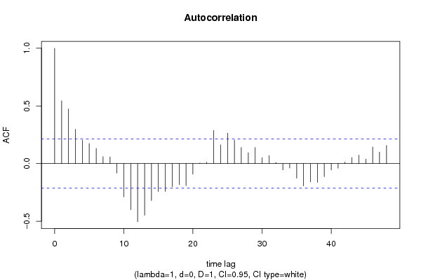
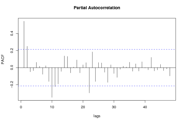
Title produced by software

(Partial) Autocorrelation Function

Date of computation

Tue, 21 Dec 2010 10:40:43 +0000

Cite this page as follows

Statistical Computations at FreeStatistics.org, Office for Research Development and Education, URL https://freestatistics.org/blog/index.php?v=date/2010/Dec/21/t1292927921sa5nhi82m35g90b.htm/, Retrieved Sat, 18 May 2024 08:35:48 +0000

Statistical Computations at FreeStatistics.org, Office for Research Development and Education, URL https://freestatistics.org/blog/index.php?pk=113245, Retrieved Sat, 18 May 2024 08:35:48 +0000

QR Codes:

Paste this QR Code to cite your computation.

Original text written by user:

IsPrivate?

No (this computation is public)

User-defined keywords

Estimated Impact

140

Family? (F = Feedback message, R = changed R code, M = changed R Module, P = changed Parameters, D = changed Data)

-     [Univariate Data Series] [] [2008-12-08 19:22:39] [d2d412c7f4d35ffbf5ee5ee89db327d4]
F RMP   [(Partial) Autocorrelation Function] [WS 9] [2010-12-07 20:24:41] [9b13650c94c5192ca5135ec8a1fa39f7]
-    D    [(Partial) Autocorrelation Function] [ACF Paper] [2010-12-19 13:35:17] [9b13650c94c5192ca5135ec8a1fa39f7]
-   P       [(Partial) Autocorrelation Function] [] [2010-12-21 10:32:09] [9b13650c94c5192ca5135ec8a1fa39f7]
-             [(Partial) Autocorrelation Function] [] [2010-12-21 10:39:04] [9b13650c94c5192ca5135ec8a1fa39f7]
-   P             [(Partial) Autocorrelation Function] [] [2010-12-21 10:40:43] [5fd8c857995b7937a45335fd5ccccdde] [Current]
-   P               [(Partial) Autocorrelation Function] [] [2010-12-21 10:50:06] [9b13650c94c5192ca5135ec8a1fa39f7] 
- RMP                 [Spectral Analysis] [] [2010-12-21 11:01:31] [9b13650c94c5192ca5135ec8a1fa39f7] 
-   P                   [Spectral Analysis] [] [2010-12-21 11:12:16] [9b13650c94c5192ca5135ec8a1fa39f7] 
-   P                     [Spectral Analysis] [] [2010-12-21 11:21:27] [9b13650c94c5192ca5135ec8a1fa39f7] 
- RMP                       [Variance Reduction Matrix] [] [2010-12-21 11:45:42] [9b13650c94c5192ca5135ec8a1fa39f7] 
- RM                          [Standard Deviation-Mean Plot] [] [2010-12-21 12:07:57] [9b13650c94c5192ca5135ec8a1fa39f7] 
- RM                          [ARIMA Backward Selection] [] [2010-12-21 12:35:49] [9b13650c94c5192ca5135ec8a1fa39f7] 
- RMP                           [ARIMA Forecasting] [] [2010-12-22 19:05:16] [9b13650c94c5192ca5135ec8a1fa39f7] 
-   P                             [ARIMA Forecasting] [] [2010-12-22 19:15:24] [9b13650c94c5192ca5135ec8a1fa39f7] 

Feedback Forum

Post a new message

Dataseries X:

Download CSV

Histogram

Boxplots

Summary of computational transaction
Raw Input	view raw input (R code)
Raw Output	view raw output of R engine
Computing time	2 seconds
R Server	'Sir Ronald Aylmer Fisher' @ 193.190.124.24

\begin{tabular}{lllllllll}
\hline
Summary of computational transaction \tabularnewline
Raw Input & view raw input (R code)  \tabularnewline
Raw Output & view raw output of R engine  \tabularnewline
Computing time & 2 seconds \tabularnewline
R Server & 'Sir Ronald Aylmer Fisher' @ 193.190.124.24 \tabularnewline
\hline
\end{tabular}
%Source: https://freestatistics.org/blog/index.php?pk=113245&T=0

[TABLE]
[ROW][C]Summary of computational transaction[/C][/ROW]
[ROW][C]Raw Input[/C][C]view raw input (R code) [/C][/ROW]
[ROW][C]Raw Output[/C][C]view raw output of R engine [/C][/ROW]
[ROW][C]Computing time[/C][C]2 seconds[/C][/ROW]
[ROW][C]R Server[/C][C]'Sir Ronald Aylmer Fisher' @ 193.190.124.24[/C][/ROW]
[/TABLE]
Source: https://freestatistics.org/blog/index.php?pk=113245&T=0

Globally Unique Identifier (entire table): ba.freestatistics.org/blog/index.php?pk=113245&T=0

As an alternative you can also use a QR Code:

The GUIDs for individual cells are displayed in the table below:

Summary of computational transaction
Raw Input	view raw input (R code)
Raw Output	view raw output of R engine
Computing time	2 seconds
R Server	'Sir Ronald Aylmer Fisher' @ 193.190.124.24

Autocorrelation Function
Time lag k	ACF(k)	T-STAT	P-value
1	0.544333	4.9889	2e-06
2	0.472879	4.334	2e-05
3	0.297398	2.7257	0.003904
4	0.203612	1.8661	0.032756
5	0.174815	1.6022	0.056432
6	0.132249	1.2121	0.11444
7	0.059772	0.5478	0.292635
8	0.058245	0.5338	0.297437
9	-0.083241	-0.7629	0.223825
10	-0.288717	-2.6461	0.004859
11	-0.399799	-3.6642	0.000217
12	-0.503688	-4.6164	7e-06
13	-0.448537	-4.1109	4.6e-05
14	-0.321273	-2.9445	0.002091
15	-0.2415	-2.2134	0.014791
16	-0.241587	-2.2142	0.014763
17	-0.200425	-1.8369	0.034879
18	-0.182912	-1.6764	0.048687
19	-0.191131	-1.7517	0.041734
20	-0.091566	-0.8392	0.201864
21	0.004889	0.0448	0.482183
22	0.013072	0.1198	0.452462
23	0.287216	2.6324	0.005044
24	0.162686	1.491	0.069848
25	0.263064	2.411	0.009044
26	0.204633	1.8755	0.0321
27	0.138819	1.2723	0.103389
28	0.094368	0.8649	0.194779
29	0.138856	1.2726	0.10333
30	0.050707	0.4647	0.32166
31	0.069489	0.6369	0.262969
32	0.009681	0.0887	0.464756
33	-0.055772	-0.5112	0.305291
34	-0.038038	-0.3486	0.364123
35	-0.127	-1.164	0.123865
36	-0.193743	-1.7757	0.039703
37	-0.157611	-1.4445	0.076155
38	-0.16252	-1.4895	0.070048
39	-0.1125	-1.0311	0.152731
40	-0.055593	-0.5095	0.305861
41	-0.04058	-0.3719	0.355442
42	0.013927	0.1276	0.449369
43	0.052748	0.4834	0.315018
44	0.074656	0.6842	0.247854
45	0.039147	0.3588	0.360327
46	0.142992	1.3105	0.096792
47	0.100271	0.919	0.180364
48	0.15683	1.4374	0.077164

\begin{tabular}{lllllllll}
\hline
Autocorrelation Function \tabularnewline
Time lag k & ACF(k) & T-STAT & P-value \tabularnewline
1 & 0.544333 & 4.9889 & 2e-06 \tabularnewline
2 & 0.472879 & 4.334 & 2e-05 \tabularnewline
3 & 0.297398 & 2.7257 & 0.003904 \tabularnewline
4 & 0.203612 & 1.8661 & 0.032756 \tabularnewline
5 & 0.174815 & 1.6022 & 0.056432 \tabularnewline
6 & 0.132249 & 1.2121 & 0.11444 \tabularnewline
7 & 0.059772 & 0.5478 & 0.292635 \tabularnewline
8 & 0.058245 & 0.5338 & 0.297437 \tabularnewline
9 & -0.083241 & -0.7629 & 0.223825 \tabularnewline
10 & -0.288717 & -2.6461 & 0.004859 \tabularnewline
11 & -0.399799 & -3.6642 & 0.000217 \tabularnewline
12 & -0.503688 & -4.6164 & 7e-06 \tabularnewline
13 & -0.448537 & -4.1109 & 4.6e-05 \tabularnewline
14 & -0.321273 & -2.9445 & 0.002091 \tabularnewline
15 & -0.2415 & -2.2134 & 0.014791 \tabularnewline
16 & -0.241587 & -2.2142 & 0.014763 \tabularnewline
17 & -0.200425 & -1.8369 & 0.034879 \tabularnewline
18 & -0.182912 & -1.6764 & 0.048687 \tabularnewline
19 & -0.191131 & -1.7517 & 0.041734 \tabularnewline
20 & -0.091566 & -0.8392 & 0.201864 \tabularnewline
21 & 0.004889 & 0.0448 & 0.482183 \tabularnewline
22 & 0.013072 & 0.1198 & 0.452462 \tabularnewline
23 & 0.287216 & 2.6324 & 0.005044 \tabularnewline
24 & 0.162686 & 1.491 & 0.069848 \tabularnewline
25 & 0.263064 & 2.411 & 0.009044 \tabularnewline
26 & 0.204633 & 1.8755 & 0.0321 \tabularnewline
27 & 0.138819 & 1.2723 & 0.103389 \tabularnewline
28 & 0.094368 & 0.8649 & 0.194779 \tabularnewline
29 & 0.138856 & 1.2726 & 0.10333 \tabularnewline
30 & 0.050707 & 0.4647 & 0.32166 \tabularnewline
31 & 0.069489 & 0.6369 & 0.262969 \tabularnewline
32 & 0.009681 & 0.0887 & 0.464756 \tabularnewline
33 & -0.055772 & -0.5112 & 0.305291 \tabularnewline
34 & -0.038038 & -0.3486 & 0.364123 \tabularnewline
35 & -0.127 & -1.164 & 0.123865 \tabularnewline
36 & -0.193743 & -1.7757 & 0.039703 \tabularnewline
37 & -0.157611 & -1.4445 & 0.076155 \tabularnewline
38 & -0.16252 & -1.4895 & 0.070048 \tabularnewline
39 & -0.1125 & -1.0311 & 0.152731 \tabularnewline
40 & -0.055593 & -0.5095 & 0.305861 \tabularnewline
41 & -0.04058 & -0.3719 & 0.355442 \tabularnewline
42 & 0.013927 & 0.1276 & 0.449369 \tabularnewline
43 & 0.052748 & 0.4834 & 0.315018 \tabularnewline
44 & 0.074656 & 0.6842 & 0.247854 \tabularnewline
45 & 0.039147 & 0.3588 & 0.360327 \tabularnewline
46 & 0.142992 & 1.3105 & 0.096792 \tabularnewline
47 & 0.100271 & 0.919 & 0.180364 \tabularnewline
48 & 0.15683 & 1.4374 & 0.077164 \tabularnewline
\hline
\end{tabular}
%Source: https://freestatistics.org/blog/index.php?pk=113245&T=1

[TABLE]
[ROW][C]Autocorrelation Function[/C][/ROW]
[ROW][C]Time lag k[/C][C]ACF(k)[/C][C]T-STAT[/C][C]P-value[/C][/ROW]
[ROW][C]1[/C][C]0.544333[/C][C]4.9889[/C][C]2e-06[/C][/ROW]
[ROW][C]2[/C][C]0.472879[/C][C]4.334[/C][C]2e-05[/C][/ROW]
[ROW][C]3[/C][C]0.297398[/C][C]2.7257[/C][C]0.003904[/C][/ROW]
[ROW][C]4[/C][C]0.203612[/C][C]1.8661[/C][C]0.032756[/C][/ROW]
[ROW][C]5[/C][C]0.174815[/C][C]1.6022[/C][C]0.056432[/C][/ROW]
[ROW][C]6[/C][C]0.132249[/C][C]1.2121[/C][C]0.11444[/C][/ROW]
[ROW][C]7[/C][C]0.059772[/C][C]0.5478[/C][C]0.292635[/C][/ROW]
[ROW][C]8[/C][C]0.058245[/C][C]0.5338[/C][C]0.297437[/C][/ROW]
[ROW][C]9[/C][C]-0.083241[/C][C]-0.7629[/C][C]0.223825[/C][/ROW]
[ROW][C]10[/C][C]-0.288717[/C][C]-2.6461[/C][C]0.004859[/C][/ROW]
[ROW][C]11[/C][C]-0.399799[/C][C]-3.6642[/C][C]0.000217[/C][/ROW]
[ROW][C]12[/C][C]-0.503688[/C][C]-4.6164[/C][C]7e-06[/C][/ROW]
[ROW][C]13[/C][C]-0.448537[/C][C]-4.1109[/C][C]4.6e-05[/C][/ROW]
[ROW][C]14[/C][C]-0.321273[/C][C]-2.9445[/C][C]0.002091[/C][/ROW]
[ROW][C]15[/C][C]-0.2415[/C][C]-2.2134[/C][C]0.014791[/C][/ROW]
[ROW][C]16[/C][C]-0.241587[/C][C]-2.2142[/C][C]0.014763[/C][/ROW]
[ROW][C]17[/C][C]-0.200425[/C][C]-1.8369[/C][C]0.034879[/C][/ROW]
[ROW][C]18[/C][C]-0.182912[/C][C]-1.6764[/C][C]0.048687[/C][/ROW]
[ROW][C]19[/C][C]-0.191131[/C][C]-1.7517[/C][C]0.041734[/C][/ROW]
[ROW][C]20[/C][C]-0.091566[/C][C]-0.8392[/C][C]0.201864[/C][/ROW]
[ROW][C]21[/C][C]0.004889[/C][C]0.0448[/C][C]0.482183[/C][/ROW]
[ROW][C]22[/C][C]0.013072[/C][C]0.1198[/C][C]0.452462[/C][/ROW]
[ROW][C]23[/C][C]0.287216[/C][C]2.6324[/C][C]0.005044[/C][/ROW]
[ROW][C]24[/C][C]0.162686[/C][C]1.491[/C][C]0.069848[/C][/ROW]
[ROW][C]25[/C][C]0.263064[/C][C]2.411[/C][C]0.009044[/C][/ROW]
[ROW][C]26[/C][C]0.204633[/C][C]1.8755[/C][C]0.0321[/C][/ROW]
[ROW][C]27[/C][C]0.138819[/C][C]1.2723[/C][C]0.103389[/C][/ROW]
[ROW][C]28[/C][C]0.094368[/C][C]0.8649[/C][C]0.194779[/C][/ROW]
[ROW][C]29[/C][C]0.138856[/C][C]1.2726[/C][C]0.10333[/C][/ROW]
[ROW][C]30[/C][C]0.050707[/C][C]0.4647[/C][C]0.32166[/C][/ROW]
[ROW][C]31[/C][C]0.069489[/C][C]0.6369[/C][C]0.262969[/C][/ROW]
[ROW][C]32[/C][C]0.009681[/C][C]0.0887[/C][C]0.464756[/C][/ROW]
[ROW][C]33[/C][C]-0.055772[/C][C]-0.5112[/C][C]0.305291[/C][/ROW]
[ROW][C]34[/C][C]-0.038038[/C][C]-0.3486[/C][C]0.364123[/C][/ROW]
[ROW][C]35[/C][C]-0.127[/C][C]-1.164[/C][C]0.123865[/C][/ROW]
[ROW][C]36[/C][C]-0.193743[/C][C]-1.7757[/C][C]0.039703[/C][/ROW]
[ROW][C]37[/C][C]-0.157611[/C][C]-1.4445[/C][C]0.076155[/C][/ROW]
[ROW][C]38[/C][C]-0.16252[/C][C]-1.4895[/C][C]0.070048[/C][/ROW]
[ROW][C]39[/C][C]-0.1125[/C][C]-1.0311[/C][C]0.152731[/C][/ROW]
[ROW][C]40[/C][C]-0.055593[/C][C]-0.5095[/C][C]0.305861[/C][/ROW]
[ROW][C]41[/C][C]-0.04058[/C][C]-0.3719[/C][C]0.355442[/C][/ROW]
[ROW][C]42[/C][C]0.013927[/C][C]0.1276[/C][C]0.449369[/C][/ROW]
[ROW][C]43[/C][C]0.052748[/C][C]0.4834[/C][C]0.315018[/C][/ROW]
[ROW][C]44[/C][C]0.074656[/C][C]0.6842[/C][C]0.247854[/C][/ROW]
[ROW][C]45[/C][C]0.039147[/C][C]0.3588[/C][C]0.360327[/C][/ROW]
[ROW][C]46[/C][C]0.142992[/C][C]1.3105[/C][C]0.096792[/C][/ROW]
[ROW][C]47[/C][C]0.100271[/C][C]0.919[/C][C]0.180364[/C][/ROW]
[ROW][C]48[/C][C]0.15683[/C][C]1.4374[/C][C]0.077164[/C][/ROW]
[/TABLE]
Source: https://freestatistics.org/blog/index.php?pk=113245&T=1

Globally Unique Identifier (entire table): ba.freestatistics.org/blog/index.php?pk=113245&T=1

As an alternative you can also use a QR Code:

The GUIDs for individual cells are displayed in the table below:

Autocorrelation Function
Time lag k	ACF(k)	T-STAT	P-value
1	0.544333	4.9889	2e-06
2	0.472879	4.334	2e-05
3	0.297398	2.7257	0.003904
4	0.203612	1.8661	0.032756
5	0.174815	1.6022	0.056432
6	0.132249	1.2121	0.11444
7	0.059772	0.5478	0.292635
8	0.058245	0.5338	0.297437
9	-0.083241	-0.7629	0.223825
10	-0.288717	-2.6461	0.004859
11	-0.399799	-3.6642	0.000217
12	-0.503688	-4.6164	7e-06
13	-0.448537	-4.1109	4.6e-05
14	-0.321273	-2.9445	0.002091
15	-0.2415	-2.2134	0.014791
16	-0.241587	-2.2142	0.014763
17	-0.200425	-1.8369	0.034879
18	-0.182912	-1.6764	0.048687
19	-0.191131	-1.7517	0.041734
20	-0.091566	-0.8392	0.201864
21	0.004889	0.0448	0.482183
22	0.013072	0.1198	0.452462
23	0.287216	2.6324	0.005044
24	0.162686	1.491	0.069848
25	0.263064	2.411	0.009044
26	0.204633	1.8755	0.0321
27	0.138819	1.2723	0.103389
28	0.094368	0.8649	0.194779
29	0.138856	1.2726	0.10333
30	0.050707	0.4647	0.32166
31	0.069489	0.6369	0.262969
32	0.009681	0.0887	0.464756
33	-0.055772	-0.5112	0.305291
34	-0.038038	-0.3486	0.364123
35	-0.127	-1.164	0.123865
36	-0.193743	-1.7757	0.039703
37	-0.157611	-1.4445	0.076155
38	-0.16252	-1.4895	0.070048
39	-0.1125	-1.0311	0.152731
40	-0.055593	-0.5095	0.305861
41	-0.04058	-0.3719	0.355442
42	0.013927	0.1276	0.449369
43	0.052748	0.4834	0.315018
44	0.074656	0.6842	0.247854
45	0.039147	0.3588	0.360327
46	0.142992	1.3105	0.096792
47	0.100271	0.919	0.180364
48	0.15683	1.4374	0.077164

Partial Autocorrelation Function
Time lag k	PACF(k)	T-STAT	P-value
1	0.544333	4.9889	2e-06
2	0.250931	2.2998	0.011969
3	-0.048537	-0.4449	0.328786
4	-0.034765	-0.3186	0.3754
5	0.062886	0.5764	0.282957
6	0.017202	0.1577	0.437551
7	-0.07791	-0.7141	0.238584
8	0.022681	0.2079	0.417914
9	-0.162152	-1.4861	0.070492
10	-0.347967	-3.1892	0.001003
11	-0.221938	-2.0341	0.022549
12	-0.191375	-1.754	0.041541
13	-0.044277	-0.4058	0.34296
14	0.137479	1.26	0.105577
15	0.132082	1.2106	0.114732
16	-0.060595	-0.5554	0.290062
17	0.007149	0.0655	0.473956
18	0.090619	0.8305	0.204295
19	-0.061212	-0.561	0.28814
20	0.03376	0.3094	0.378884
21	0.058976	0.5405	0.295134
22	-0.295694	-2.7101	0.004077
23	0.184509	1.6911	0.047267
24	-0.162177	-1.4864	0.070461
25	0.060291	0.5526	0.29101
26	0.056235	0.5154	0.303814
27	-0.054102	-0.4959	0.310645
28	-0.172354	-1.5797	0.058972
29	0.03369	0.3088	0.379129
30	-0.068081	-0.624	0.267169
31	-0.114605	-1.0504	0.14828
32	-0.018849	-0.1728	0.431631
33	0.017453	0.16	0.436649
34	0.007951	0.0729	0.471041
35	0.063981	0.5864	0.27959
36	-0.042521	-0.3897	0.348868
37	0.045667	0.4185	0.33831
38	-0.039577	-0.3627	0.358858
39	0.068724	0.6299	0.265245
40	-0.002959	-0.0271	0.489213
41	-0.025539	-0.2341	0.407749
42	0.121129	1.1102	0.135047
43	-0.03856	-0.3534	0.362335
44	-0.026617	-0.2439	0.403933
45	0.037982	0.3481	0.364313
46	-0.035143	-0.3221	0.374093
47	-0.014074	-0.129	0.448836
48	-0.096624	-0.8856	0.189189

\begin{tabular}{lllllllll}
\hline
Partial Autocorrelation Function \tabularnewline
Time lag k & PACF(k) & T-STAT & P-value \tabularnewline
1 & 0.544333 & 4.9889 & 2e-06 \tabularnewline
2 & 0.250931 & 2.2998 & 0.011969 \tabularnewline
3 & -0.048537 & -0.4449 & 0.328786 \tabularnewline
4 & -0.034765 & -0.3186 & 0.3754 \tabularnewline
5 & 0.062886 & 0.5764 & 0.282957 \tabularnewline
6 & 0.017202 & 0.1577 & 0.437551 \tabularnewline
7 & -0.07791 & -0.7141 & 0.238584 \tabularnewline
8 & 0.022681 & 0.2079 & 0.417914 \tabularnewline
9 & -0.162152 & -1.4861 & 0.070492 \tabularnewline
10 & -0.347967 & -3.1892 & 0.001003 \tabularnewline
11 & -0.221938 & -2.0341 & 0.022549 \tabularnewline
12 & -0.191375 & -1.754 & 0.041541 \tabularnewline
13 & -0.044277 & -0.4058 & 0.34296 \tabularnewline
14 & 0.137479 & 1.26 & 0.105577 \tabularnewline
15 & 0.132082 & 1.2106 & 0.114732 \tabularnewline
16 & -0.060595 & -0.5554 & 0.290062 \tabularnewline
17 & 0.007149 & 0.0655 & 0.473956 \tabularnewline
18 & 0.090619 & 0.8305 & 0.204295 \tabularnewline
19 & -0.061212 & -0.561 & 0.28814 \tabularnewline
20 & 0.03376 & 0.3094 & 0.378884 \tabularnewline
21 & 0.058976 & 0.5405 & 0.295134 \tabularnewline
22 & -0.295694 & -2.7101 & 0.004077 \tabularnewline
23 & 0.184509 & 1.6911 & 0.047267 \tabularnewline
24 & -0.162177 & -1.4864 & 0.070461 \tabularnewline
25 & 0.060291 & 0.5526 & 0.29101 \tabularnewline
26 & 0.056235 & 0.5154 & 0.303814 \tabularnewline
27 & -0.054102 & -0.4959 & 0.310645 \tabularnewline
28 & -0.172354 & -1.5797 & 0.058972 \tabularnewline
29 & 0.03369 & 0.3088 & 0.379129 \tabularnewline
30 & -0.068081 & -0.624 & 0.267169 \tabularnewline
31 & -0.114605 & -1.0504 & 0.14828 \tabularnewline
32 & -0.018849 & -0.1728 & 0.431631 \tabularnewline
33 & 0.017453 & 0.16 & 0.436649 \tabularnewline
34 & 0.007951 & 0.0729 & 0.471041 \tabularnewline
35 & 0.063981 & 0.5864 & 0.27959 \tabularnewline
36 & -0.042521 & -0.3897 & 0.348868 \tabularnewline
37 & 0.045667 & 0.4185 & 0.33831 \tabularnewline
38 & -0.039577 & -0.3627 & 0.358858 \tabularnewline
39 & 0.068724 & 0.6299 & 0.265245 \tabularnewline
40 & -0.002959 & -0.0271 & 0.489213 \tabularnewline
41 & -0.025539 & -0.2341 & 0.407749 \tabularnewline
42 & 0.121129 & 1.1102 & 0.135047 \tabularnewline
43 & -0.03856 & -0.3534 & 0.362335 \tabularnewline
44 & -0.026617 & -0.2439 & 0.403933 \tabularnewline
45 & 0.037982 & 0.3481 & 0.364313 \tabularnewline
46 & -0.035143 & -0.3221 & 0.374093 \tabularnewline
47 & -0.014074 & -0.129 & 0.448836 \tabularnewline
48 & -0.096624 & -0.8856 & 0.189189 \tabularnewline
\hline
\end{tabular}
%Source: https://freestatistics.org/blog/index.php?pk=113245&T=2

[TABLE]
[ROW][C]Partial Autocorrelation Function[/C][/ROW]
[ROW][C]Time lag k[/C][C]PACF(k)[/C][C]T-STAT[/C][C]P-value[/C][/ROW]
[ROW][C]1[/C][C]0.544333[/C][C]4.9889[/C][C]2e-06[/C][/ROW]
[ROW][C]2[/C][C]0.250931[/C][C]2.2998[/C][C]0.011969[/C][/ROW]
[ROW][C]3[/C][C]-0.048537[/C][C]-0.4449[/C][C]0.328786[/C][/ROW]
[ROW][C]4[/C][C]-0.034765[/C][C]-0.3186[/C][C]0.3754[/C][/ROW]
[ROW][C]5[/C][C]0.062886[/C][C]0.5764[/C][C]0.282957[/C][/ROW]
[ROW][C]6[/C][C]0.017202[/C][C]0.1577[/C][C]0.437551[/C][/ROW]
[ROW][C]7[/C][C]-0.07791[/C][C]-0.7141[/C][C]0.238584[/C][/ROW]
[ROW][C]8[/C][C]0.022681[/C][C]0.2079[/C][C]0.417914[/C][/ROW]
[ROW][C]9[/C][C]-0.162152[/C][C]-1.4861[/C][C]0.070492[/C][/ROW]
[ROW][C]10[/C][C]-0.347967[/C][C]-3.1892[/C][C]0.001003[/C][/ROW]
[ROW][C]11[/C][C]-0.221938[/C][C]-2.0341[/C][C]0.022549[/C][/ROW]
[ROW][C]12[/C][C]-0.191375[/C][C]-1.754[/C][C]0.041541[/C][/ROW]
[ROW][C]13[/C][C]-0.044277[/C][C]-0.4058[/C][C]0.34296[/C][/ROW]
[ROW][C]14[/C][C]0.137479[/C][C]1.26[/C][C]0.105577[/C][/ROW]
[ROW][C]15[/C][C]0.132082[/C][C]1.2106[/C][C]0.114732[/C][/ROW]
[ROW][C]16[/C][C]-0.060595[/C][C]-0.5554[/C][C]0.290062[/C][/ROW]
[ROW][C]17[/C][C]0.007149[/C][C]0.0655[/C][C]0.473956[/C][/ROW]
[ROW][C]18[/C][C]0.090619[/C][C]0.8305[/C][C]0.204295[/C][/ROW]
[ROW][C]19[/C][C]-0.061212[/C][C]-0.561[/C][C]0.28814[/C][/ROW]
[ROW][C]20[/C][C]0.03376[/C][C]0.3094[/C][C]0.378884[/C][/ROW]
[ROW][C]21[/C][C]0.058976[/C][C]0.5405[/C][C]0.295134[/C][/ROW]
[ROW][C]22[/C][C]-0.295694[/C][C]-2.7101[/C][C]0.004077[/C][/ROW]
[ROW][C]23[/C][C]0.184509[/C][C]1.6911[/C][C]0.047267[/C][/ROW]
[ROW][C]24[/C][C]-0.162177[/C][C]-1.4864[/C][C]0.070461[/C][/ROW]
[ROW][C]25[/C][C]0.060291[/C][C]0.5526[/C][C]0.29101[/C][/ROW]
[ROW][C]26[/C][C]0.056235[/C][C]0.5154[/C][C]0.303814[/C][/ROW]
[ROW][C]27[/C][C]-0.054102[/C][C]-0.4959[/C][C]0.310645[/C][/ROW]
[ROW][C]28[/C][C]-0.172354[/C][C]-1.5797[/C][C]0.058972[/C][/ROW]
[ROW][C]29[/C][C]0.03369[/C][C]0.3088[/C][C]0.379129[/C][/ROW]
[ROW][C]30[/C][C]-0.068081[/C][C]-0.624[/C][C]0.267169[/C][/ROW]
[ROW][C]31[/C][C]-0.114605[/C][C]-1.0504[/C][C]0.14828[/C][/ROW]
[ROW][C]32[/C][C]-0.018849[/C][C]-0.1728[/C][C]0.431631[/C][/ROW]
[ROW][C]33[/C][C]0.017453[/C][C]0.16[/C][C]0.436649[/C][/ROW]
[ROW][C]34[/C][C]0.007951[/C][C]0.0729[/C][C]0.471041[/C][/ROW]
[ROW][C]35[/C][C]0.063981[/C][C]0.5864[/C][C]0.27959[/C][/ROW]
[ROW][C]36[/C][C]-0.042521[/C][C]-0.3897[/C][C]0.348868[/C][/ROW]
[ROW][C]37[/C][C]0.045667[/C][C]0.4185[/C][C]0.33831[/C][/ROW]
[ROW][C]38[/C][C]-0.039577[/C][C]-0.3627[/C][C]0.358858[/C][/ROW]
[ROW][C]39[/C][C]0.068724[/C][C]0.6299[/C][C]0.265245[/C][/ROW]
[ROW][C]40[/C][C]-0.002959[/C][C]-0.0271[/C][C]0.489213[/C][/ROW]
[ROW][C]41[/C][C]-0.025539[/C][C]-0.2341[/C][C]0.407749[/C][/ROW]
[ROW][C]42[/C][C]0.121129[/C][C]1.1102[/C][C]0.135047[/C][/ROW]
[ROW][C]43[/C][C]-0.03856[/C][C]-0.3534[/C][C]0.362335[/C][/ROW]
[ROW][C]44[/C][C]-0.026617[/C][C]-0.2439[/C][C]0.403933[/C][/ROW]
[ROW][C]45[/C][C]0.037982[/C][C]0.3481[/C][C]0.364313[/C][/ROW]
[ROW][C]46[/C][C]-0.035143[/C][C]-0.3221[/C][C]0.374093[/C][/ROW]
[ROW][C]47[/C][C]-0.014074[/C][C]-0.129[/C][C]0.448836[/C][/ROW]
[ROW][C]48[/C][C]-0.096624[/C][C]-0.8856[/C][C]0.189189[/C][/ROW]
[/TABLE]
Source: https://freestatistics.org/blog/index.php?pk=113245&T=2

Globally Unique Identifier (entire table): ba.freestatistics.org/blog/index.php?pk=113245&T=2

As an alternative you can also use a QR Code:

The GUIDs for individual cells are displayed in the table below:

Partial Autocorrelation Function
Time lag k	PACF(k)	T-STAT	P-value
1	0.544333	4.9889	2e-06
2	0.250931	2.2998	0.011969
3	-0.048537	-0.4449	0.328786
4	-0.034765	-0.3186	0.3754
5	0.062886	0.5764	0.282957
6	0.017202	0.1577	0.437551
7	-0.07791	-0.7141	0.238584
8	0.022681	0.2079	0.417914
9	-0.162152	-1.4861	0.070492
10	-0.347967	-3.1892	0.001003
11	-0.221938	-2.0341	0.022549
12	-0.191375	-1.754	0.041541
13	-0.044277	-0.4058	0.34296
14	0.137479	1.26	0.105577
15	0.132082	1.2106	0.114732
16	-0.060595	-0.5554	0.290062
17	0.007149	0.0655	0.473956
18	0.090619	0.8305	0.204295
19	-0.061212	-0.561	0.28814
20	0.03376	0.3094	0.378884
21	0.058976	0.5405	0.295134
22	-0.295694	-2.7101	0.004077
23	0.184509	1.6911	0.047267
24	-0.162177	-1.4864	0.070461
25	0.060291	0.5526	0.29101
26	0.056235	0.5154	0.303814
27	-0.054102	-0.4959	0.310645
28	-0.172354	-1.5797	0.058972
29	0.03369	0.3088	0.379129
30	-0.068081	-0.624	0.267169
31	-0.114605	-1.0504	0.14828
32	-0.018849	-0.1728	0.431631
33	0.017453	0.16	0.436649
34	0.007951	0.0729	0.471041
35	0.063981	0.5864	0.27959
36	-0.042521	-0.3897	0.348868
37	0.045667	0.4185	0.33831
38	-0.039577	-0.3627	0.358858
39	0.068724	0.6299	0.265245
40	-0.002959	-0.0271	0.489213
41	-0.025539	-0.2341	0.407749
42	0.121129	1.1102	0.135047
43	-0.03856	-0.3534	0.362335
44	-0.026617	-0.2439	0.403933
45	0.037982	0.3481	0.364313
46	-0.035143	-0.3221	0.374093
47	-0.014074	-0.129	0.448836
48	-0.096624	-0.8856	0.189189

Figure 1

PNG link

Postscript link

PDF link

Figure 2

PNG link

Postscript link

PDF link

Parameters (Session):

par1 = 48 ; par2 = 1 ; par3 = 0 ; par4 = 1 ; par5 = 12 ; par6 = White Noise ; par7 = 0.95 ;

Parameters (R input):

par1 = 48 ; par2 = 1 ; par3 = 0 ; par4 = 1 ; par5 = 12 ; par6 = White Noise ; par7 = 0.95 ; par8 = ;

R code (references can be found in the software module):

if (par1 == 'Default') {
par1 = 10*log10(length(x))
} else {
par1 <- as.numeric(par1)
}
par2 <- as.numeric(par2)
par3 <- as.numeric(par3)
par4 <- as.numeric(par4)
par5 <- as.numeric(par5)
if (par6 == 'White Noise') par6 <- 'white' else par6 <- 'ma'
par7 <- as.numeric(par7)
if (par2 == 0) {
x <- log(x)
} else {
x <- (x ^ par2 - 1) / par2
}
if (par3 > 0) x <- diff(x,lag=1,difference=par3)
if (par4 > 0) x <- diff(x,lag=par5,difference=par4)
bitmap(file='pic1.png')
racf <- acf(x, par1, main='Autocorrelation', xlab='time lag', ylab='ACF', ci.type=par6, ci=par7, sub=paste('(lambda=',par2,', d=',par3,', D=',par4,', CI=', par7, ', CI type=',par6,')',sep=''))
dev.off()
bitmap(file='pic2.png')
rpacf <- pacf(x,par1,main='Partial Autocorrelation',xlab='lags',ylab='PACF')
dev.off()
(myacf <- c(racf$acf))
(mypacf <- c(rpacf$acf))
lengthx <- length(x)
sqrtn <- sqrt(lengthx)
load(file='createtable')
a<-table.start()
a<-table.row.start(a)
a<-table.element(a,'Autocorrelation Function',4,TRUE)
a<-table.row.end(a)
a<-table.row.start(a)
a<-table.element(a,'Time lag k',header=TRUE)
a<-table.element(a,hyperlink('basics.htm','ACF(k)','click here for more information about the Autocorrelation Function'),header=TRUE)
a<-table.element(a,'T-STAT',header=TRUE)
a<-table.element(a,'P-value',header=TRUE)
a<-table.row.end(a)
for (i in 2:(par1+1)) {
a<-table.row.start(a)
a<-table.element(a,i-1,header=TRUE)
a<-table.element(a,round(myacf[i],6))
mytstat <- myacf[i]*sqrtn
a<-table.element(a,round(mytstat,4))
a<-table.element(a,round(1-pt(abs(mytstat),lengthx),6))
a<-table.row.end(a)
}
a<-table.end(a)
table.save(a,file='mytable.tab')
a<-table.start()
a<-table.row.start(a)
a<-table.element(a,'Partial Autocorrelation Function',4,TRUE)
a<-table.row.end(a)
a<-table.row.start(a)
a<-table.element(a,'Time lag k',header=TRUE)
a<-table.element(a,hyperlink('basics.htm','PACF(k)','click here for more information about the Partial Autocorrelation Function'),header=TRUE)
a<-table.element(a,'T-STAT',header=TRUE)
a<-table.element(a,'P-value',header=TRUE)
a<-table.row.end(a)
for (i in 1:par1) {
a<-table.row.start(a)
a<-table.element(a,i,header=TRUE)
a<-table.element(a,round(mypacf[i],6))
mytstat <- mypacf[i]*sqrtn
a<-table.element(a,round(mytstat,4))
a<-table.element(a,round(1-pt(abs(mytstat),lengthx),6))
a<-table.row.end(a)
}
a<-table.end(a)
table.save(a,file='mytable1.tab')

Free Statistics

Description of Statistical Computation

Tree of Dependent Computations

Dataset

Tables (Output of Computation)

Figures (Output of Computation)

Input Parameters & R Code