Free Statistics
of Irreproducible Research!
Description of Statistical Computation | |||||||||||||||||||||||||||||||||||||
|---|---|---|---|---|---|---|---|---|---|---|---|---|---|---|---|---|---|---|---|---|---|---|---|---|---|---|---|---|---|---|---|---|---|---|---|---|---|
| Author's title | |||||||||||||||||||||||||||||||||||||
| Author | *The author of this computation has been verified* | ||||||||||||||||||||||||||||||||||||
| R Software Module | rwasp_boxcoxnorm.wasp | ||||||||||||||||||||||||||||||||||||
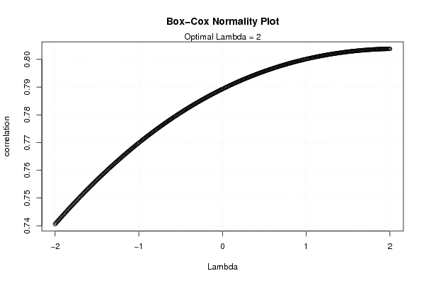
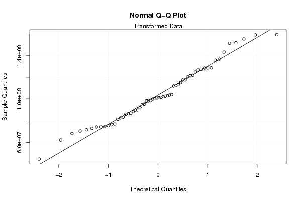
| Title produced by software | Box-Cox Normality Plot | ||||||||||||||||||||||||||||||||||||
| Date of computation | Tue, 11 Nov 2008 10:40:11 -0700 | ||||||||||||||||||||||||||||||||||||
| Cite this page as follows | Statistical Computations at FreeStatistics.org, Office for Research Development and Education, URL https://freestatistics.org/blog/index.php?v=date/2008/Nov/11/t1226425264scav5mhuqk6uzpm.htm/, Retrieved Wed, 15 May 2024 18:00:14 +0000 | ||||||||||||||||||||||||||||||||||||
| Statistical Computations at FreeStatistics.org, Office for Research Development and Education, URL https://freestatistics.org/blog/index.php?pk=23771, Retrieved Wed, 15 May 2024 18:00:14 +0000 | |||||||||||||||||||||||||||||||||||||
| QR Codes: | |||||||||||||||||||||||||||||||||||||
|
| |||||||||||||||||||||||||||||||||||||
| Original text written by user: | |||||||||||||||||||||||||||||||||||||
| IsPrivate? | No (this computation is public) | ||||||||||||||||||||||||||||||||||||
| User-defined keywords | |||||||||||||||||||||||||||||||||||||
| Estimated Impact | 155 | ||||||||||||||||||||||||||||||||||||
Tree of Dependent Computations | |||||||||||||||||||||||||||||||||||||
| Family? (F = Feedback message, R = changed R code, M = changed R Module, P = changed Parameters, D = changed Data) | |||||||||||||||||||||||||||||||||||||
| - [Bivariate Kernel Density Estimation] [Q1 Bivariate Dens...] [2007-11-03 14:50:57] [e2ec4dc832988c648c062d4cdc574d44] - RMPD [Hierarchical Clustering] [WS4 Q2 dendrogram] [2007-11-05 10:02:49] [74be16979710d4c4e7c6647856088456] - RMPD [Box-Cox Normality Plot] [various eda topic...] [2008-11-04 20:30:40] [077ffec662d24c06be4c491541a44245] F D [Box-Cox Normality Plot] [various eda topic...] [2008-11-04 20:48:12] [077ffec662d24c06be4c491541a44245] F P [Box-Cox Normality Plot] [Box-Cox Normality...] [2008-11-11 16:08:06] [73d6180dc45497329efd1b6934a84aba] F [Box-Cox Normality Plot] [Box-Cox Normality...] [2008-11-11 17:40:11] [14a75ec03b2c0d8ddd8b141a7b1594fd] [Current] F [Box-Cox Normality Plot] [] [2008-11-11 20:04:58] [a7a7b7de998247cdf0f65ef79d563d66] - [Box-Cox Normality Plot] [] [2008-11-21 18:02:08] [888addc516c3b812dd7be4bd54caa358] | |||||||||||||||||||||||||||||||||||||
| Feedback Forum | |||||||||||||||||||||||||||||||||||||
Post a new message | |||||||||||||||||||||||||||||||||||||
Dataset | |||||||||||||||||||||||||||||||||||||
| Dataseries X: | |||||||||||||||||||||||||||||||||||||
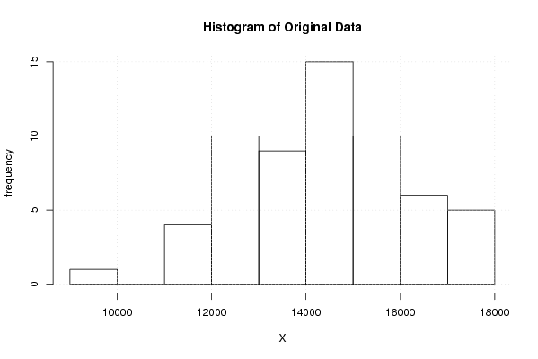
12300.00 12092.80 12380.80 12196.90 9455.00 13168.00 13427.90 11980.50 11884.80 11691.70 12233.80 14341.40 13130.70 12421.10 14285.80 12864.60 11160.20 14316.20 14388.70 14013.90 13419.00 12769.60 13315.50 15332.90 14243.00 13824.40 14962.90 13202.90 12199.00 15508.90 14199.80 15169.60 14058.00 13786.20 14147.90 16541.70 13587.50 15582.40 15802.80 14130.50 12923.20 15612.20 16033.70 16036.60 14037.80 15330.60 15038.30 17401.80 14992.50 16043.70 16929.60 15921.30 14417.20 15961.00 17851.90 16483.90 14215.50 17429.70 17839.50 17629.20 | |||||||||||||||||||||||||||||||||||||
Tables (Output of Computation) | |||||||||||||||||||||||||||||||||||||
| |||||||||||||||||||||||||||||||||||||
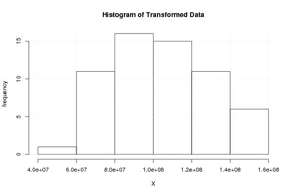
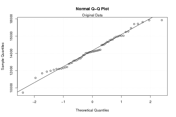
Figures (Output of Computation) | |||||||||||||||||||||||||||||||||||||
Input Parameters & R Code | |||||||||||||||||||||||||||||||||||||
| Parameters (Session): | |||||||||||||||||||||||||||||||||||||
| par1 = 50 ; par2 = 50 ; par3 = Y ; par4 = Y ; par5 = uitvoer Vlaanderen ; par6 = uitvoer Belgie naar landen buiten EU ; par7 = uitvoer Belgie (totaal) ; | |||||||||||||||||||||||||||||||||||||
| Parameters (R input): | |||||||||||||||||||||||||||||||||||||
| R code (references can be found in the software module): | |||||||||||||||||||||||||||||||||||||
n <- length(x) | |||||||||||||||||||||||||||||||||||||