Free Statistics
of Irreproducible Research!
Description of Statistical Computation | |||||||||||||||||||||||||||||||||||||
|---|---|---|---|---|---|---|---|---|---|---|---|---|---|---|---|---|---|---|---|---|---|---|---|---|---|---|---|---|---|---|---|---|---|---|---|---|---|
| Author's title | |||||||||||||||||||||||||||||||||||||
| Author | *The author of this computation has been verified* | ||||||||||||||||||||||||||||||||||||
| R Software Module | rwasp_boxcoxnorm.wasp | ||||||||||||||||||||||||||||||||||||
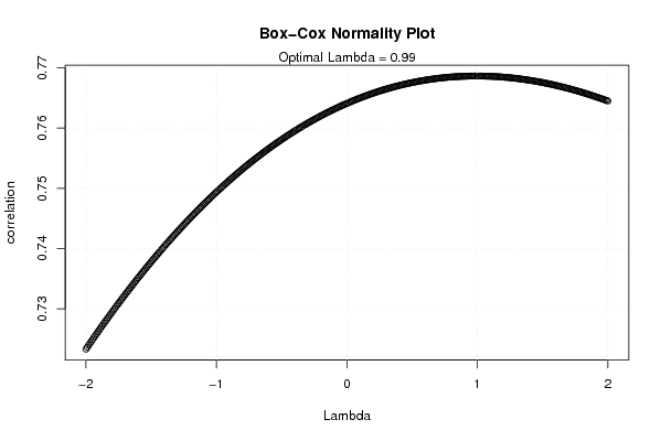
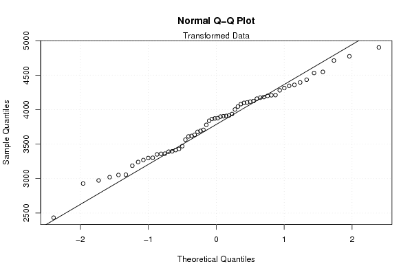
| Title produced by software | Box-Cox Normality Plot | ||||||||||||||||||||||||||||||||||||
| Date of computation | Tue, 04 Nov 2008 13:30:40 -0700 | ||||||||||||||||||||||||||||||||||||
| Cite this page as follows | Statistical Computations at FreeStatistics.org, Office for Research Development and Education, URL https://freestatistics.org/blog/index.php?v=date/2008/Nov/04/t12258307103hfc5ehcbzs509g.htm/, Retrieved Wed, 15 May 2024 06:47:25 +0000 | ||||||||||||||||||||||||||||||||||||
| Statistical Computations at FreeStatistics.org, Office for Research Development and Education, URL https://freestatistics.org/blog/index.php?pk=21656, Retrieved Wed, 15 May 2024 06:47:25 +0000 | |||||||||||||||||||||||||||||||||||||
| QR Codes: | |||||||||||||||||||||||||||||||||||||
|
| |||||||||||||||||||||||||||||||||||||
| Original text written by user: | |||||||||||||||||||||||||||||||||||||
| IsPrivate? | No (this computation is public) | ||||||||||||||||||||||||||||||||||||
| User-defined keywords | |||||||||||||||||||||||||||||||||||||
| Estimated Impact | 205 | ||||||||||||||||||||||||||||||||||||
Tree of Dependent Computations | |||||||||||||||||||||||||||||||||||||
| Family? (F = Feedback message, R = changed R code, M = changed R Module, P = changed Parameters, D = changed Data) | |||||||||||||||||||||||||||||||||||||
| - [Bivariate Kernel Density Estimation] [Q1 Bivariate Dens...] [2007-11-03 14:50:57] [e2ec4dc832988c648c062d4cdc574d44] - RMPD [Hierarchical Clustering] [WS4 Q2 dendrogram] [2007-11-05 10:02:49] [74be16979710d4c4e7c6647856088456] - RMPD [Box-Cox Normality Plot] [various eda topic...] [2008-11-04 20:30:40] [3817f5e632a8bfeb1be7b5e8c86bd450] [Current] F D [Box-Cox Normality Plot] [various eda topic...] [2008-11-04 20:48:12] [077ffec662d24c06be4c491541a44245] F PD [Box-Cox Normality Plot] [] [2008-11-09 18:41:47] [4c8dfb519edec2da3492d7e6be9a5685] F P [Box-Cox Normality Plot] [Box-Cox Normality...] [2008-11-11 16:08:06] [73d6180dc45497329efd1b6934a84aba] F [Box-Cox Normality Plot] [Box-Cox Normality...] [2008-11-11 17:40:11] [6816386b1f3c2f6c0c9f2aa1e5bc9362] F [Box-Cox Normality Plot] [] [2008-11-11 20:04:58] [a7a7b7de998247cdf0f65ef79d563d66] - [Box-Cox Normality Plot] [] [2008-11-21 18:02:08] [888addc516c3b812dd7be4bd54caa358] | |||||||||||||||||||||||||||||||||||||
| Feedback Forum | |||||||||||||||||||||||||||||||||||||
Post a new message | |||||||||||||||||||||||||||||||||||||
Dataset | |||||||||||||||||||||||||||||||||||||
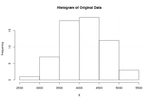
| Dataseries X: | |||||||||||||||||||||||||||||||||||||
3423.40 3242.80 3277.20 3833.00 2606.30 3643.80 3686.40 3281.60 3669.30 3191.50 3512.70 3970.70 3601.20 3610.00 4172.10 3956.20 3142.70 3884.30 3892.20 3613.00 3730.50 3481.30 3649.50 4215.20 4066.60 4196.80 4536.60 4441.60 3548.30 4735.90 4130.60 4356.20 4159.60 3988.00 4167.80 4902.20 3909.40 4697.60 4308.90 4420.40 3544.20 4433.00 4479.70 4533.20 4237.50 4207.40 4394.00 5148.40 4202.20 4682.50 4884.30 5288.90 4505.20 4611.50 5081.10 4523.10 4412.80 4647.40 4778.60 4495.30 | |||||||||||||||||||||||||||||||||||||
Tables (Output of Computation) | |||||||||||||||||||||||||||||||||||||
| |||||||||||||||||||||||||||||||||||||
Figures (Output of Computation) | |||||||||||||||||||||||||||||||||||||
Input Parameters & R Code | |||||||||||||||||||||||||||||||||||||
| Parameters (Session): | |||||||||||||||||||||||||||||||||||||
| par1 = TRUE ; | |||||||||||||||||||||||||||||||||||||
| Parameters (R input): | |||||||||||||||||||||||||||||||||||||
| R code (references can be found in the software module): | |||||||||||||||||||||||||||||||||||||
n <- length(x) | |||||||||||||||||||||||||||||||||||||