Repository of Reproducible Computations

Free Statistics

of Irreproducible Research!

Author's title

Author

*The author of this computation has been verified*

R Software Module

rwasp_autocorrelation.wasp

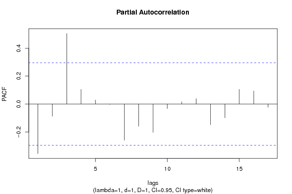
Title produced by software

(Partial) Autocorrelation Function

Date of computation

Sat, 25 Dec 2010 10:28:55 +0000

Cite this page as follows

Statistical Computations at FreeStatistics.org, Office for Research Development and Education, URL https://freestatistics.org/blog/index.php?v=date/2010/Dec/25/t12932729395rrv3jhi2ntsftl.htm/, Retrieved Mon, 29 Apr 2024 00:49:41 +0000

Statistical Computations at FreeStatistics.org, Office for Research Development and Education, URL https://freestatistics.org/blog/index.php?pk=115345, Retrieved Mon, 29 Apr 2024 00:49:41 +0000

QR Codes:

Paste this QR Code to cite your computation.

Original text written by user:

IsPrivate?

No (this computation is public)

User-defined keywords

Estimated Impact

184

Family? (F = Feedback message, R = changed R code, M = changed R Module, P = changed Parameters, D = changed Data)

F     [(Partial) Autocorrelation Function] [(P)ACF Algemeen i...] [2008-12-03 16:58:16] [74be16979710d4c4e7c6647856088456]
- RMPD    [(Partial) Autocorrelation Function] [paper (P)ACF gedi...] [2010-12-25 10:28:55] [b7765ad69c3ab250b1ef04c2ab1247ec] [Current]
-   P       [(Partial) Autocorrelation Function] [Gedifferentieerde...] [2010-12-26 11:47:51] [c4f608d390ad7371b1365a9b84541edb] 
-   P         [(Partial) Autocorrelation Function] [Gedifferentieerde...] [2010-12-26 13:27:39] [c4f608d390ad7371b1365a9b84541edb] 
-               [(Partial) Autocorrelation Function] [Gedifferentieerde...] [2010-12-29 19:57:03] [7c2d060fd17a41a80970d273bf259e67] 
-               [(Partial) Autocorrelation Function] [] [2010-12-29 20:07:55] [a2638725f7f7c6bd63902ba17eba666b] 
-               [(Partial) Autocorrelation Function] [gediff tijdreeks] [2010-12-29 22:04:32] [df61ce38492c371f14c407a12b3bb2eb] 

Feedback Forum

Post a new message

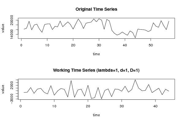
Dataseries X:

Download CSV

Histogram

Boxplots

Summary of computational transaction
Raw Input	view raw input (R code)
Raw Output	view raw output of R engine
Computing time	2 seconds
R Server	'Gwilym Jenkins' @ 72.249.127.135

\begin{tabular}{lllllllll}
\hline
Summary of computational transaction \tabularnewline
Raw Input & view raw input (R code)  \tabularnewline
Raw Output & view raw output of R engine  \tabularnewline
Computing time & 2 seconds \tabularnewline
R Server & 'Gwilym Jenkins' @ 72.249.127.135 \tabularnewline
\hline
\end{tabular}
%Source: https://freestatistics.org/blog/index.php?pk=115345&T=0

[TABLE]
[ROW][C]Summary of computational transaction[/C][/ROW]
[ROW][C]Raw Input[/C][C]view raw input (R code) [/C][/ROW]
[ROW][C]Raw Output[/C][C]view raw output of R engine [/C][/ROW]
[ROW][C]Computing time[/C][C]2 seconds[/C][/ROW]
[ROW][C]R Server[/C][C]'Gwilym Jenkins' @ 72.249.127.135[/C][/ROW]
[/TABLE]
Source: https://freestatistics.org/blog/index.php?pk=115345&T=0

Globally Unique Identifier (entire table): ba.freestatistics.org/blog/index.php?pk=115345&T=0

As an alternative you can also use a QR Code:

The GUIDs for individual cells are displayed in the table below:

Summary of computational transaction
Raw Input	view raw input (R code)
Raw Output	view raw output of R engine
Computing time	2 seconds
R Server	'Gwilym Jenkins' @ 72.249.127.135

Autocorrelation Function
Time lag k	ACF(k)	T-STAT	P-value
1	-0.355101	-2.3555	0.011511
2	0.049435	0.3279	0.372267
3	0.450301	2.987	0.002296
4	-0.260388	-1.7272	0.045571
5	0.153904	1.0209	0.156445
6	0.15383	1.0204	0.15656
7	-0.300179	-1.9912	0.026347
8	0.168034	1.1146	0.135535
9	-0.11603	-0.7697	0.222809
10	-0.135399	-0.8981	0.187001
11	0.06993	0.4639	0.322515
12	-0.161356	-1.0703	0.145158
13	-0.1427	-0.9466	0.174516
14	0.062991	0.4178	0.33905
15	-0.069133	-0.4586	0.324397
16	-0.065154	-0.4322	0.333861
17	0.004619	0.0306	0.487848

\begin{tabular}{lllllllll}
\hline
Autocorrelation Function \tabularnewline
Time lag k & ACF(k) & T-STAT & P-value \tabularnewline
1 & -0.355101 & -2.3555 & 0.011511 \tabularnewline
2 & 0.049435 & 0.3279 & 0.372267 \tabularnewline
3 & 0.450301 & 2.987 & 0.002296 \tabularnewline
4 & -0.260388 & -1.7272 & 0.045571 \tabularnewline
5 & 0.153904 & 1.0209 & 0.156445 \tabularnewline
6 & 0.15383 & 1.0204 & 0.15656 \tabularnewline
7 & -0.300179 & -1.9912 & 0.026347 \tabularnewline
8 & 0.168034 & 1.1146 & 0.135535 \tabularnewline
9 & -0.11603 & -0.7697 & 0.222809 \tabularnewline
10 & -0.135399 & -0.8981 & 0.187001 \tabularnewline
11 & 0.06993 & 0.4639 & 0.322515 \tabularnewline
12 & -0.161356 & -1.0703 & 0.145158 \tabularnewline
13 & -0.1427 & -0.9466 & 0.174516 \tabularnewline
14 & 0.062991 & 0.4178 & 0.33905 \tabularnewline
15 & -0.069133 & -0.4586 & 0.324397 \tabularnewline
16 & -0.065154 & -0.4322 & 0.333861 \tabularnewline
17 & 0.004619 & 0.0306 & 0.487848 \tabularnewline
\hline
\end{tabular}
%Source: https://freestatistics.org/blog/index.php?pk=115345&T=1

[TABLE]
[ROW][C]Autocorrelation Function[/C][/ROW]
[ROW][C]Time lag k[/C][C]ACF(k)[/C][C]T-STAT[/C][C]P-value[/C][/ROW]
[ROW][C]1[/C][C]-0.355101[/C][C]-2.3555[/C][C]0.011511[/C][/ROW]
[ROW][C]2[/C][C]0.049435[/C][C]0.3279[/C][C]0.372267[/C][/ROW]
[ROW][C]3[/C][C]0.450301[/C][C]2.987[/C][C]0.002296[/C][/ROW]
[ROW][C]4[/C][C]-0.260388[/C][C]-1.7272[/C][C]0.045571[/C][/ROW]
[ROW][C]5[/C][C]0.153904[/C][C]1.0209[/C][C]0.156445[/C][/ROW]
[ROW][C]6[/C][C]0.15383[/C][C]1.0204[/C][C]0.15656[/C][/ROW]
[ROW][C]7[/C][C]-0.300179[/C][C]-1.9912[/C][C]0.026347[/C][/ROW]
[ROW][C]8[/C][C]0.168034[/C][C]1.1146[/C][C]0.135535[/C][/ROW]
[ROW][C]9[/C][C]-0.11603[/C][C]-0.7697[/C][C]0.222809[/C][/ROW]
[ROW][C]10[/C][C]-0.135399[/C][C]-0.8981[/C][C]0.187001[/C][/ROW]
[ROW][C]11[/C][C]0.06993[/C][C]0.4639[/C][C]0.322515[/C][/ROW]
[ROW][C]12[/C][C]-0.161356[/C][C]-1.0703[/C][C]0.145158[/C][/ROW]
[ROW][C]13[/C][C]-0.1427[/C][C]-0.9466[/C][C]0.174516[/C][/ROW]
[ROW][C]14[/C][C]0.062991[/C][C]0.4178[/C][C]0.33905[/C][/ROW]
[ROW][C]15[/C][C]-0.069133[/C][C]-0.4586[/C][C]0.324397[/C][/ROW]
[ROW][C]16[/C][C]-0.065154[/C][C]-0.4322[/C][C]0.333861[/C][/ROW]
[ROW][C]17[/C][C]0.004619[/C][C]0.0306[/C][C]0.487848[/C][/ROW]
[/TABLE]
Source: https://freestatistics.org/blog/index.php?pk=115345&T=1

Globally Unique Identifier (entire table): ba.freestatistics.org/blog/index.php?pk=115345&T=1

As an alternative you can also use a QR Code:

The GUIDs for individual cells are displayed in the table below:

Autocorrelation Function
Time lag k	ACF(k)	T-STAT	P-value
1	-0.355101	-2.3555	0.011511
2	0.049435	0.3279	0.372267
3	0.450301	2.987	0.002296
4	-0.260388	-1.7272	0.045571
5	0.153904	1.0209	0.156445
6	0.15383	1.0204	0.15656
7	-0.300179	-1.9912	0.026347
8	0.168034	1.1146	0.135535
9	-0.11603	-0.7697	0.222809
10	-0.135399	-0.8981	0.187001
11	0.06993	0.4639	0.322515
12	-0.161356	-1.0703	0.145158
13	-0.1427	-0.9466	0.174516
14	0.062991	0.4178	0.33905
15	-0.069133	-0.4586	0.324397
16	-0.065154	-0.4322	0.333861
17	0.004619	0.0306	0.487848

Partial Autocorrelation Function
Time lag k	PACF(k)	T-STAT	P-value
1	-0.355101	-2.3555	0.011511
2	-0.087724	-0.5819	0.281803
3	0.505368	3.3522	0.000828
4	0.104881	0.6957	0.245137
5	0.028559	0.1894	0.42531
6	-0.003108	-0.0206	0.491823
7	-0.259668	-1.7224	0.046006
8	-0.159452	-1.0577	0.147986
9	-0.203845	-1.3522	0.091618
10	-0.033448	-0.2219	0.412722
11	0.015733	0.1044	0.458679
12	0.038779	0.2572	0.3991
13	-0.148481	-0.9849	0.165027
14	-0.099109	-0.6574	0.257169
15	0.105288	0.6984	0.2443
16	0.09371	0.6216	0.268706
17	-0.023306	-0.1546	0.438924

\begin{tabular}{lllllllll}
\hline
Partial Autocorrelation Function \tabularnewline
Time lag k & PACF(k) & T-STAT & P-value \tabularnewline
1 & -0.355101 & -2.3555 & 0.011511 \tabularnewline
2 & -0.087724 & -0.5819 & 0.281803 \tabularnewline
3 & 0.505368 & 3.3522 & 0.000828 \tabularnewline
4 & 0.104881 & 0.6957 & 0.245137 \tabularnewline
5 & 0.028559 & 0.1894 & 0.42531 \tabularnewline
6 & -0.003108 & -0.0206 & 0.491823 \tabularnewline
7 & -0.259668 & -1.7224 & 0.046006 \tabularnewline
8 & -0.159452 & -1.0577 & 0.147986 \tabularnewline
9 & -0.203845 & -1.3522 & 0.091618 \tabularnewline
10 & -0.033448 & -0.2219 & 0.412722 \tabularnewline
11 & 0.015733 & 0.1044 & 0.458679 \tabularnewline
12 & 0.038779 & 0.2572 & 0.3991 \tabularnewline
13 & -0.148481 & -0.9849 & 0.165027 \tabularnewline
14 & -0.099109 & -0.6574 & 0.257169 \tabularnewline
15 & 0.105288 & 0.6984 & 0.2443 \tabularnewline
16 & 0.09371 & 0.6216 & 0.268706 \tabularnewline
17 & -0.023306 & -0.1546 & 0.438924 \tabularnewline
\hline
\end{tabular}
%Source: https://freestatistics.org/blog/index.php?pk=115345&T=2

[TABLE]
[ROW][C]Partial Autocorrelation Function[/C][/ROW]
[ROW][C]Time lag k[/C][C]PACF(k)[/C][C]T-STAT[/C][C]P-value[/C][/ROW]
[ROW][C]1[/C][C]-0.355101[/C][C]-2.3555[/C][C]0.011511[/C][/ROW]
[ROW][C]2[/C][C]-0.087724[/C][C]-0.5819[/C][C]0.281803[/C][/ROW]
[ROW][C]3[/C][C]0.505368[/C][C]3.3522[/C][C]0.000828[/C][/ROW]
[ROW][C]4[/C][C]0.104881[/C][C]0.6957[/C][C]0.245137[/C][/ROW]
[ROW][C]5[/C][C]0.028559[/C][C]0.1894[/C][C]0.42531[/C][/ROW]
[ROW][C]6[/C][C]-0.003108[/C][C]-0.0206[/C][C]0.491823[/C][/ROW]
[ROW][C]7[/C][C]-0.259668[/C][C]-1.7224[/C][C]0.046006[/C][/ROW]
[ROW][C]8[/C][C]-0.159452[/C][C]-1.0577[/C][C]0.147986[/C][/ROW]
[ROW][C]9[/C][C]-0.203845[/C][C]-1.3522[/C][C]0.091618[/C][/ROW]
[ROW][C]10[/C][C]-0.033448[/C][C]-0.2219[/C][C]0.412722[/C][/ROW]
[ROW][C]11[/C][C]0.015733[/C][C]0.1044[/C][C]0.458679[/C][/ROW]
[ROW][C]12[/C][C]0.038779[/C][C]0.2572[/C][C]0.3991[/C][/ROW]
[ROW][C]13[/C][C]-0.148481[/C][C]-0.9849[/C][C]0.165027[/C][/ROW]
[ROW][C]14[/C][C]-0.099109[/C][C]-0.6574[/C][C]0.257169[/C][/ROW]
[ROW][C]15[/C][C]0.105288[/C][C]0.6984[/C][C]0.2443[/C][/ROW]
[ROW][C]16[/C][C]0.09371[/C][C]0.6216[/C][C]0.268706[/C][/ROW]
[ROW][C]17[/C][C]-0.023306[/C][C]-0.1546[/C][C]0.438924[/C][/ROW]
[/TABLE]
Source: https://freestatistics.org/blog/index.php?pk=115345&T=2

Globally Unique Identifier (entire table): ba.freestatistics.org/blog/index.php?pk=115345&T=2

As an alternative you can also use a QR Code:

The GUIDs for individual cells are displayed in the table below:

Partial Autocorrelation Function
Time lag k	PACF(k)	T-STAT	P-value
1	-0.355101	-2.3555	0.011511
2	-0.087724	-0.5819	0.281803
3	0.505368	3.3522	0.000828
4	0.104881	0.6957	0.245137
5	0.028559	0.1894	0.42531
6	-0.003108	-0.0206	0.491823
7	-0.259668	-1.7224	0.046006
8	-0.159452	-1.0577	0.147986
9	-0.203845	-1.3522	0.091618
10	-0.033448	-0.2219	0.412722
11	0.015733	0.1044	0.458679
12	0.038779	0.2572	0.3991
13	-0.148481	-0.9849	0.165027
14	-0.099109	-0.6574	0.257169
15	0.105288	0.6984	0.2443
16	0.09371	0.6216	0.268706
17	-0.023306	-0.1546	0.438924

Figure 1

PNG link

Postscript link

PDF link

Figure 2

PNG link

Postscript link

PDF link

Figure 3

PNG link

Postscript link

PDF link

Parameters (Session):

par1 = Default ; par2 = 1 ; par3 = 1 ; par4 = 1 ; par5 = 12 ; par6 = White Noise ; par7 = 0.95 ;

Parameters (R input):

par1 = Default ; par2 = 1 ; par3 = 1 ; par4 = 1 ; par5 = 12 ; par6 = White Noise ; par7 = 0.95 ; par8 = ;

R code (references can be found in the software module):

if (par1 == 'Default') {
par1 = 10*log10(length(x))
} else {
par1 <- as.numeric(par1)
}
par2 <- as.numeric(par2)
par3 <- as.numeric(par3)
par4 <- as.numeric(par4)
par5 <- as.numeric(par5)
if (par6 == 'White Noise') par6 <- 'white' else par6 <- 'ma'
par7 <- as.numeric(par7)
if (par8 != '') par8 <- as.numeric(par8)
ox <- x
if (par8 == '') {
if (par2 == 0) {
x <- log(x)
} else {
x <- (x ^ par2 - 1) / par2
}
} else {
x <- log(x,base=par8)
}
if (par3 > 0) x <- diff(x,lag=1,difference=par3)
if (par4 > 0) x <- diff(x,lag=par5,difference=par4)
bitmap(file='picts.png')
op <- par(mfrow=c(2,1))
plot(ox,type='l',main='Original Time Series',xlab='time',ylab='value')
if (par8=='') {
mytitle <- paste('Working Time Series (lambda=',par2,', d=',par3,', D=',par4,')',sep='')
mysub <- paste('(lambda=',par2,', d=',par3,', D=',par4,', CI=', par7, ', CI type=',par6,')',sep='')
} else {
mytitle <- paste('Working Time Series (base=',par8,', d=',par3,', D=',par4,')',sep='')
mysub <- paste('(base=',par8,', d=',par3,', D=',par4,', CI=', par7, ', CI type=',par6,')',sep='')
}
plot(x,type='l', main=mytitle,xlab='time',ylab='value')
par(op)
dev.off()
bitmap(file='pic1.png')
racf <- acf(x, par1, main='Autocorrelation', xlab='time lag', ylab='ACF', ci.type=par6, ci=par7, sub=mysub)
dev.off()
bitmap(file='pic2.png')
rpacf <- pacf(x,par1,main='Partial Autocorrelation',xlab='lags',ylab='PACF',sub=mysub)
dev.off()
(myacf <- c(racf$acf))
(mypacf <- c(rpacf$acf))
lengthx <- length(x)
sqrtn <- sqrt(lengthx)
load(file='createtable')
a<-table.start()
a<-table.row.start(a)
a<-table.element(a,'Autocorrelation Function',4,TRUE)
a<-table.row.end(a)
a<-table.row.start(a)
a<-table.element(a,'Time lag k',header=TRUE)
a<-table.element(a,hyperlink('basics.htm','ACF(k)','click here for more information about the Autocorrelation Function'),header=TRUE)
a<-table.element(a,'T-STAT',header=TRUE)
a<-table.element(a,'P-value',header=TRUE)
a<-table.row.end(a)
for (i in 2:(par1+1)) {
a<-table.row.start(a)
a<-table.element(a,i-1,header=TRUE)
a<-table.element(a,round(myacf[i],6))
mytstat <- myacf[i]*sqrtn
a<-table.element(a,round(mytstat,4))
a<-table.element(a,round(1-pt(abs(mytstat),lengthx),6))
a<-table.row.end(a)
}
a<-table.end(a)
table.save(a,file='mytable.tab')
a<-table.start()
a<-table.row.start(a)
a<-table.element(a,'Partial Autocorrelation Function',4,TRUE)
a<-table.row.end(a)
a<-table.row.start(a)
a<-table.element(a,'Time lag k',header=TRUE)
a<-table.element(a,hyperlink('basics.htm','PACF(k)','click here for more information about the Partial Autocorrelation Function'),header=TRUE)
a<-table.element(a,'T-STAT',header=TRUE)
a<-table.element(a,'P-value',header=TRUE)
a<-table.row.end(a)
for (i in 1:par1) {
a<-table.row.start(a)
a<-table.element(a,i,header=TRUE)
a<-table.element(a,round(mypacf[i],6))
mytstat <- mypacf[i]*sqrtn
a<-table.element(a,round(mytstat,4))
a<-table.element(a,round(1-pt(abs(mytstat),lengthx),6))
a<-table.row.end(a)
}
a<-table.end(a)
table.save(a,file='mytable1.tab')

Free Statistics

Description of Statistical Computation

Tree of Dependent Computations

Dataset

Tables (Output of Computation)

Figures (Output of Computation)

Input Parameters & R Code