Repository of Reproducible Computations

Free Statistics

of Irreproducible Research!

Author's title

Author

*Unverified author*

R Software Module

rwasp_autocorrelation.wasp

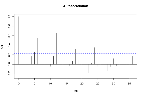
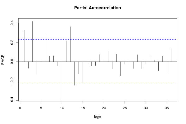
Title produced by software

(Partial) Autocorrelation Function

Date of computation

Wed, 03 Dec 2008 09:58:16 -0700

Cite this page as follows

Statistical Computations at FreeStatistics.org, Office for Research Development and Education, URL https://freestatistics.org/blog/index.php?v=date/2008/Dec/03/t1228323645tmxqg3su20rzc4u.htm/, Retrieved Mon, 13 May 2024 23:01:58 +0000

Statistical Computations at FreeStatistics.org, Office for Research Development and Education, URL https://freestatistics.org/blog/index.php?pk=28795, Retrieved Mon, 13 May 2024 23:01:58 +0000

QR Codes:

Paste this QR Code to cite your computation.

Original text written by user:

IsPrivate?

No (this computation is public)

User-defined keywords

Estimated Impact

242

Family? (F = Feedback message, R = changed R code, M = changed R Module, P = changed Parameters, D = changed Data)

F       [(Partial) Autocorrelation Function] [(P)ACF Algemeen i...] [2008-12-03 16:58:16] [d41d8cd98f00b204e9800998ecf8427e] [Current]
- RMPD    [(Partial) Autocorrelation Function] [paper (p)ACF] [2010-12-25 09:05:34] [df61ce38492c371f14c407a12b3bb2eb] 
-    D      [(Partial) Autocorrelation Function] [] [2010-12-26 09:57:06] [a2638725f7f7c6bd63902ba17eba666b] 
-   P       [(Partial) Autocorrelation Function] [] [2010-12-26 10:56:45] [c4f608d390ad7371b1365a9b84541edb] 
- RMPD    [Variance Reduction Matrix] [paper VRM] [2010-12-25 09:11:26] [df61ce38492c371f14c407a12b3bb2eb] 
- RMPD    [Spectral Analysis] [paper periodogrammen] [2010-12-25 09:34:41] [df61ce38492c371f14c407a12b3bb2eb] 
-   P       [Spectral Analysis] [paper periodogrammen] [2010-12-25 11:37:30] [df61ce38492c371f14c407a12b3bb2eb] 
-   P         [Spectral Analysis] [spectral analysis] [2010-12-26 11:44:40] [c4f608d390ad7371b1365a9b84541edb] 
-   P         [Spectral Analysis] [spectral analysis] [2010-12-26 13:19:56] [c4f608d390ad7371b1365a9b84541edb] 
-               [Spectral Analysis] [Spectral Analysis] [2010-12-29 19:53:36] [7c2d060fd17a41a80970d273bf259e67] 
-               [Spectral Analysis] [] [2010-12-29 20:03:47] [a2638725f7f7c6bd63902ba17eba666b] 
-               [Spectral Analysis] [spec analyse] [2010-12-29 21:57:35] [df61ce38492c371f14c407a12b3bb2eb] 
-           [Spectral Analysis] [spectral analysis] [2010-12-28 10:11:41] [c4f608d390ad7371b1365a9b84541edb] 
-           [Spectral Analysis] [Gedifferentieerde...] [2010-12-28 10:11:41] [c4f608d390ad7371b1365a9b84541edb] 
-           [Spectral Analysis] [Periodogrammen] [2010-12-29 19:58:49] [7c2d060fd17a41a80970d273bf259e67] 
-           [Spectral Analysis] [] [2010-12-29 20:10:11] [a2638725f7f7c6bd63902ba17eba666b] 
-           [Spectral Analysis] [periodogrammen] [2010-12-29 22:06:28] [df61ce38492c371f14c407a12b3bb2eb] 
- RMPD    [Standard Deviation-Mean Plot] [paper SD mean plot] [2010-12-25 09:54:12] [df61ce38492c371f14c407a12b3bb2eb] 
-           [Standard Deviation-Mean Plot] [standard deviatio...] [2010-12-28 10:08:05] [c4f608d390ad7371b1365a9b84541edb] 
-           [Standard Deviation-Mean Plot] [Standard Deviatio...] [2010-12-29 19:55:38] [7c2d060fd17a41a80970d273bf259e67] 
-           [Standard Deviation-Mean Plot] [] [2010-12-29 20:06:12] [a2638725f7f7c6bd63902ba17eba666b] 
-           [Standard Deviation-Mean Plot] [SDMP] [2010-12-29 21:59:27] [df61ce38492c371f14c407a12b3bb2eb] 
- RMPD    [(Partial) Autocorrelation Function] [paper (P)ACF gedi...] [2010-12-25 10:28:55] [df61ce38492c371f14c407a12b3bb2eb] 
-   P       [(Partial) Autocorrelation Function] [Gedifferentieerde...] [2010-12-26 11:47:51] [c4f608d390ad7371b1365a9b84541edb] 
-   P         [(Partial) Autocorrelation Function] [Gedifferentieerde...] [2010-12-26 13:27:39] [c4f608d390ad7371b1365a9b84541edb] 
-               [(Partial) Autocorrelation Function] [Gedifferentieerde...] [2010-12-29 19:57:03] [7c2d060fd17a41a80970d273bf259e67] 
-               [(Partial) Autocorrelation Function] [] [2010-12-29 20:07:55] [a2638725f7f7c6bd63902ba17eba666b] 
-               [(Partial) Autocorrelation Function] [gediff tijdreeks] [2010-12-29 22:04:32] [df61ce38492c371f14c407a12b3bb2eb] 

Feedback Forum

2008-12-13 10:52:10 [Maarten Van Gucht] [reply] 
de student heeft een goede berekening en goede conclusie gemaakt. je kan hier inderdaad zien dat er veel correlaties significant verschillend zijn, dat de meeste buiten de betrouwbaarheidsintervallen liggen. zoals de student ook vermeld in zijn antwoord moet de tijdreeks stationnair worden, dit kunnen we doen door de differentieren. je kan op de grafiek moeilijk zien hoe we moeten differentieren (seizoenaal/trendmatig) voor zeker te zijn gaan we kijken in de variantie reductie matrix.

Post a new message

Dataseries X:

Download CSV

Histogram

Boxplots

Summary of computational transaction
Raw Input	view raw input (R code)
Raw Output	view raw output of R engine
Computing time	1 seconds
R Server	'George Udny Yule' @ 72.249.76.132

\begin{tabular}{lllllllll}
\hline
Summary of computational transaction \tabularnewline
Raw Input & view raw input (R code)  \tabularnewline
Raw Output & view raw output of R engine  \tabularnewline
Computing time & 1 seconds \tabularnewline
R Server & 'George Udny Yule' @ 72.249.76.132 \tabularnewline
\hline
\end{tabular}
%Source: https://freestatistics.org/blog/index.php?pk=28795&T=0

[TABLE]
[ROW][C]Summary of computational transaction[/C][/ROW]
[ROW][C]Raw Input[/C][C]view raw input (R code) [/C][/ROW]
[ROW][C]Raw Output[/C][C]view raw output of R engine [/C][/ROW]
[ROW][C]Computing time[/C][C]1 seconds[/C][/ROW]
[ROW][C]R Server[/C][C]'George Udny Yule' @ 72.249.76.132[/C][/ROW]
[/TABLE]
Source: https://freestatistics.org/blog/index.php?pk=28795&T=0

Globally Unique Identifier (entire table): ba.freestatistics.org/blog/index.php?pk=28795&T=0

As an alternative you can also use a QR Code:

The GUIDs for individual cells are displayed in the table below:

Summary of computational transaction
Raw Input	view raw input (R code)
Raw Output	view raw output of R engine
Computing time	1 seconds
R Server	'George Udny Yule' @ 72.249.76.132

Autocorrelation Function
Time lag k	ACF(k)	T-STAT	P-value
1	0.327082	2.7946	0.003317
2	0.046708	0.3991	0.345503
3	0.364344	3.113	0.001322
4	0.168139	1.4366	0.077555
5	0.261832	2.2371	0.014167
6	0.555093	4.7427	5e-06
7	0.253831	2.1687	0.016681
8	0.133657	1.142	0.128599
9	0.267379	2.2845	0.012626
10	-0.043063	-0.3679	0.356994
11	0.180005	1.538	0.06419
12	0.651265	5.5644	0
13	0.136941	1.17	0.122898
14	-0.080562	-0.6883	0.246716
15	0.142264	1.2155	0.114045
16	-0.02723	-0.2326	0.408342
17	0.069357	0.5926	0.277645
18	0.314028	2.6831	0.004509
19	0.081984	0.7005	0.24293
20	-0.016411	-0.1402	0.444439
21	0.092743	0.7924	0.215348
22	-0.184464	-1.5761	0.059668
23	0.023218	0.1984	0.421653
24	0.352421	3.0111	0.001787
25	-0.043093	-0.3682	0.356901
26	-0.157789	-1.3481	0.09089
27	-0.018785	-0.1605	0.436466
28	-0.139622	-1.1929	0.118379
29	-0.0477	-0.4076	0.342398
30	0.120892	1.0329	0.15253
31	-0.028026	-0.2395	0.405711
32	-0.075733	-0.6471	0.259811
33	-0.0644	-0.5502	0.29192
34	-0.244053	-2.0852	0.020274
35	-0.070441	-0.6019	0.274569
36	0.169776	1.4506	0.075592

\begin{tabular}{lllllllll}
\hline
Autocorrelation Function \tabularnewline
Time lag k & ACF(k) & T-STAT & P-value \tabularnewline
1 & 0.327082 & 2.7946 & 0.003317 \tabularnewline
2 & 0.046708 & 0.3991 & 0.345503 \tabularnewline
3 & 0.364344 & 3.113 & 0.001322 \tabularnewline
4 & 0.168139 & 1.4366 & 0.077555 \tabularnewline
5 & 0.261832 & 2.2371 & 0.014167 \tabularnewline
6 & 0.555093 & 4.7427 & 5e-06 \tabularnewline
7 & 0.253831 & 2.1687 & 0.016681 \tabularnewline
8 & 0.133657 & 1.142 & 0.128599 \tabularnewline
9 & 0.267379 & 2.2845 & 0.012626 \tabularnewline
10 & -0.043063 & -0.3679 & 0.356994 \tabularnewline
11 & 0.180005 & 1.538 & 0.06419 \tabularnewline
12 & 0.651265 & 5.5644 & 0 \tabularnewline
13 & 0.136941 & 1.17 & 0.122898 \tabularnewline
14 & -0.080562 & -0.6883 & 0.246716 \tabularnewline
15 & 0.142264 & 1.2155 & 0.114045 \tabularnewline
16 & -0.02723 & -0.2326 & 0.408342 \tabularnewline
17 & 0.069357 & 0.5926 & 0.277645 \tabularnewline
18 & 0.314028 & 2.6831 & 0.004509 \tabularnewline
19 & 0.081984 & 0.7005 & 0.24293 \tabularnewline
20 & -0.016411 & -0.1402 & 0.444439 \tabularnewline
21 & 0.092743 & 0.7924 & 0.215348 \tabularnewline
22 & -0.184464 & -1.5761 & 0.059668 \tabularnewline
23 & 0.023218 & 0.1984 & 0.421653 \tabularnewline
24 & 0.352421 & 3.0111 & 0.001787 \tabularnewline
25 & -0.043093 & -0.3682 & 0.356901 \tabularnewline
26 & -0.157789 & -1.3481 & 0.09089 \tabularnewline
27 & -0.018785 & -0.1605 & 0.436466 \tabularnewline
28 & -0.139622 & -1.1929 & 0.118379 \tabularnewline
29 & -0.0477 & -0.4076 & 0.342398 \tabularnewline
30 & 0.120892 & 1.0329 & 0.15253 \tabularnewline
31 & -0.028026 & -0.2395 & 0.405711 \tabularnewline
32 & -0.075733 & -0.6471 & 0.259811 \tabularnewline
33 & -0.0644 & -0.5502 & 0.29192 \tabularnewline
34 & -0.244053 & -2.0852 & 0.020274 \tabularnewline
35 & -0.070441 & -0.6019 & 0.274569 \tabularnewline
36 & 0.169776 & 1.4506 & 0.075592 \tabularnewline
\hline
\end{tabular}
%Source: https://freestatistics.org/blog/index.php?pk=28795&T=1

[TABLE]
[ROW][C]Autocorrelation Function[/C][/ROW]
[ROW][C]Time lag k[/C][C]ACF(k)[/C][C]T-STAT[/C][C]P-value[/C][/ROW]
[ROW][C]1[/C][C]0.327082[/C][C]2.7946[/C][C]0.003317[/C][/ROW]
[ROW][C]2[/C][C]0.046708[/C][C]0.3991[/C][C]0.345503[/C][/ROW]
[ROW][C]3[/C][C]0.364344[/C][C]3.113[/C][C]0.001322[/C][/ROW]
[ROW][C]4[/C][C]0.168139[/C][C]1.4366[/C][C]0.077555[/C][/ROW]
[ROW][C]5[/C][C]0.261832[/C][C]2.2371[/C][C]0.014167[/C][/ROW]
[ROW][C]6[/C][C]0.555093[/C][C]4.7427[/C][C]5e-06[/C][/ROW]
[ROW][C]7[/C][C]0.253831[/C][C]2.1687[/C][C]0.016681[/C][/ROW]
[ROW][C]8[/C][C]0.133657[/C][C]1.142[/C][C]0.128599[/C][/ROW]
[ROW][C]9[/C][C]0.267379[/C][C]2.2845[/C][C]0.012626[/C][/ROW]
[ROW][C]10[/C][C]-0.043063[/C][C]-0.3679[/C][C]0.356994[/C][/ROW]
[ROW][C]11[/C][C]0.180005[/C][C]1.538[/C][C]0.06419[/C][/ROW]
[ROW][C]12[/C][C]0.651265[/C][C]5.5644[/C][C]0[/C][/ROW]
[ROW][C]13[/C][C]0.136941[/C][C]1.17[/C][C]0.122898[/C][/ROW]
[ROW][C]14[/C][C]-0.080562[/C][C]-0.6883[/C][C]0.246716[/C][/ROW]
[ROW][C]15[/C][C]0.142264[/C][C]1.2155[/C][C]0.114045[/C][/ROW]
[ROW][C]16[/C][C]-0.02723[/C][C]-0.2326[/C][C]0.408342[/C][/ROW]
[ROW][C]17[/C][C]0.069357[/C][C]0.5926[/C][C]0.277645[/C][/ROW]
[ROW][C]18[/C][C]0.314028[/C][C]2.6831[/C][C]0.004509[/C][/ROW]
[ROW][C]19[/C][C]0.081984[/C][C]0.7005[/C][C]0.24293[/C][/ROW]
[ROW][C]20[/C][C]-0.016411[/C][C]-0.1402[/C][C]0.444439[/C][/ROW]
[ROW][C]21[/C][C]0.092743[/C][C]0.7924[/C][C]0.215348[/C][/ROW]
[ROW][C]22[/C][C]-0.184464[/C][C]-1.5761[/C][C]0.059668[/C][/ROW]
[ROW][C]23[/C][C]0.023218[/C][C]0.1984[/C][C]0.421653[/C][/ROW]
[ROW][C]24[/C][C]0.352421[/C][C]3.0111[/C][C]0.001787[/C][/ROW]
[ROW][C]25[/C][C]-0.043093[/C][C]-0.3682[/C][C]0.356901[/C][/ROW]
[ROW][C]26[/C][C]-0.157789[/C][C]-1.3481[/C][C]0.09089[/C][/ROW]
[ROW][C]27[/C][C]-0.018785[/C][C]-0.1605[/C][C]0.436466[/C][/ROW]
[ROW][C]28[/C][C]-0.139622[/C][C]-1.1929[/C][C]0.118379[/C][/ROW]
[ROW][C]29[/C][C]-0.0477[/C][C]-0.4076[/C][C]0.342398[/C][/ROW]
[ROW][C]30[/C][C]0.120892[/C][C]1.0329[/C][C]0.15253[/C][/ROW]
[ROW][C]31[/C][C]-0.028026[/C][C]-0.2395[/C][C]0.405711[/C][/ROW]
[ROW][C]32[/C][C]-0.075733[/C][C]-0.6471[/C][C]0.259811[/C][/ROW]
[ROW][C]33[/C][C]-0.0644[/C][C]-0.5502[/C][C]0.29192[/C][/ROW]
[ROW][C]34[/C][C]-0.244053[/C][C]-2.0852[/C][C]0.020274[/C][/ROW]
[ROW][C]35[/C][C]-0.070441[/C][C]-0.6019[/C][C]0.274569[/C][/ROW]
[ROW][C]36[/C][C]0.169776[/C][C]1.4506[/C][C]0.075592[/C][/ROW]
[/TABLE]
Source: https://freestatistics.org/blog/index.php?pk=28795&T=1

Globally Unique Identifier (entire table): ba.freestatistics.org/blog/index.php?pk=28795&T=1

As an alternative you can also use a QR Code:

The GUIDs for individual cells are displayed in the table below:

Autocorrelation Function
Time lag k	ACF(k)	T-STAT	P-value
1	0.327082	2.7946	0.003317
2	0.046708	0.3991	0.345503
3	0.364344	3.113	0.001322
4	0.168139	1.4366	0.077555
5	0.261832	2.2371	0.014167
6	0.555093	4.7427	5e-06
7	0.253831	2.1687	0.016681
8	0.133657	1.142	0.128599
9	0.267379	2.2845	0.012626
10	-0.043063	-0.3679	0.356994
11	0.180005	1.538	0.06419
12	0.651265	5.5644	0
13	0.136941	1.17	0.122898
14	-0.080562	-0.6883	0.246716
15	0.142264	1.2155	0.114045
16	-0.02723	-0.2326	0.408342
17	0.069357	0.5926	0.277645
18	0.314028	2.6831	0.004509
19	0.081984	0.7005	0.24293
20	-0.016411	-0.1402	0.444439
21	0.092743	0.7924	0.215348
22	-0.184464	-1.5761	0.059668
23	0.023218	0.1984	0.421653
24	0.352421	3.0111	0.001787
25	-0.043093	-0.3682	0.356901
26	-0.157789	-1.3481	0.09089
27	-0.018785	-0.1605	0.436466
28	-0.139622	-1.1929	0.118379
29	-0.0477	-0.4076	0.342398
30	0.120892	1.0329	0.15253
31	-0.028026	-0.2395	0.405711
32	-0.075733	-0.6471	0.259811
33	-0.0644	-0.5502	0.29192
34	-0.244053	-2.0852	0.020274
35	-0.070441	-0.6019	0.274569
36	0.169776	1.4506	0.075592

Partial Autocorrelation Function
Time lag k	PACF(k)	T-STAT	P-value
1	0.327082	2.7946	0.003317
2	-0.067496	-0.5767	0.282964
3	0.416348	3.5573	0.000331
4	-0.130028	-1.111	0.135116
5	0.412125	3.5212	0.000372
6	0.291292	2.4888	0.007549
7	0.058399	0.499	0.309654
8	0.061484	0.5253	0.300476
9	-0.043952	-0.3755	0.354181
10	-0.375978	-3.2124	0.00098
11	0.216429	1.8492	0.034241
12	0.36203	3.0932	0.001403
13	-0.24277	-2.0742	0.020793
14	-0.125581	-1.073	0.14341
15	-0.214726	-1.8346	0.035318
16	-0.003937	-0.0336	0.486628
17	-0.043102	-0.3683	0.356872
18	-0.039275	-0.3356	0.369082
19	0.07403	0.6325	0.264514
20	0.006225	0.0532	0.478864
21	0.109354	0.9343	0.17661
22	-0.073644	-0.6292	0.265587
23	0.080229	0.6855	0.247607
24	-0.142518	-1.2177	0.113635
25	-0.026363	-0.2252	0.411209
26	-0.026151	-0.2234	0.41191
27	-0.070008	-0.5981	0.275797
28	0.073458	0.6276	0.266105
29	-0.071419	-0.6102	0.271811
30	-0.020902	-0.1786	0.429377
31	0.056187	0.4801	0.316311
32	0.019209	0.1641	0.435043
33	-0.092293	-0.7886	0.216463
34	0.060218	0.5145	0.304228
35	-0.116096	-0.9919	0.162256
36	0.13593	1.1614	0.124635

\begin{tabular}{lllllllll}
\hline
Partial Autocorrelation Function \tabularnewline
Time lag k & PACF(k) & T-STAT & P-value \tabularnewline
1 & 0.327082 & 2.7946 & 0.003317 \tabularnewline
2 & -0.067496 & -0.5767 & 0.282964 \tabularnewline
3 & 0.416348 & 3.5573 & 0.000331 \tabularnewline
4 & -0.130028 & -1.111 & 0.135116 \tabularnewline
5 & 0.412125 & 3.5212 & 0.000372 \tabularnewline
6 & 0.291292 & 2.4888 & 0.007549 \tabularnewline
7 & 0.058399 & 0.499 & 0.309654 \tabularnewline
8 & 0.061484 & 0.5253 & 0.300476 \tabularnewline
9 & -0.043952 & -0.3755 & 0.354181 \tabularnewline
10 & -0.375978 & -3.2124 & 0.00098 \tabularnewline
11 & 0.216429 & 1.8492 & 0.034241 \tabularnewline
12 & 0.36203 & 3.0932 & 0.001403 \tabularnewline
13 & -0.24277 & -2.0742 & 0.020793 \tabularnewline
14 & -0.125581 & -1.073 & 0.14341 \tabularnewline
15 & -0.214726 & -1.8346 & 0.035318 \tabularnewline
16 & -0.003937 & -0.0336 & 0.486628 \tabularnewline
17 & -0.043102 & -0.3683 & 0.356872 \tabularnewline
18 & -0.039275 & -0.3356 & 0.369082 \tabularnewline
19 & 0.07403 & 0.6325 & 0.264514 \tabularnewline
20 & 0.006225 & 0.0532 & 0.478864 \tabularnewline
21 & 0.109354 & 0.9343 & 0.17661 \tabularnewline
22 & -0.073644 & -0.6292 & 0.265587 \tabularnewline
23 & 0.080229 & 0.6855 & 0.247607 \tabularnewline
24 & -0.142518 & -1.2177 & 0.113635 \tabularnewline
25 & -0.026363 & -0.2252 & 0.411209 \tabularnewline
26 & -0.026151 & -0.2234 & 0.41191 \tabularnewline
27 & -0.070008 & -0.5981 & 0.275797 \tabularnewline
28 & 0.073458 & 0.6276 & 0.266105 \tabularnewline
29 & -0.071419 & -0.6102 & 0.271811 \tabularnewline
30 & -0.020902 & -0.1786 & 0.429377 \tabularnewline
31 & 0.056187 & 0.4801 & 0.316311 \tabularnewline
32 & 0.019209 & 0.1641 & 0.435043 \tabularnewline
33 & -0.092293 & -0.7886 & 0.216463 \tabularnewline
34 & 0.060218 & 0.5145 & 0.304228 \tabularnewline
35 & -0.116096 & -0.9919 & 0.162256 \tabularnewline
36 & 0.13593 & 1.1614 & 0.124635 \tabularnewline
\hline
\end{tabular}
%Source: https://freestatistics.org/blog/index.php?pk=28795&T=2

[TABLE]
[ROW][C]Partial Autocorrelation Function[/C][/ROW]
[ROW][C]Time lag k[/C][C]PACF(k)[/C][C]T-STAT[/C][C]P-value[/C][/ROW]
[ROW][C]1[/C][C]0.327082[/C][C]2.7946[/C][C]0.003317[/C][/ROW]
[ROW][C]2[/C][C]-0.067496[/C][C]-0.5767[/C][C]0.282964[/C][/ROW]
[ROW][C]3[/C][C]0.416348[/C][C]3.5573[/C][C]0.000331[/C][/ROW]
[ROW][C]4[/C][C]-0.130028[/C][C]-1.111[/C][C]0.135116[/C][/ROW]
[ROW][C]5[/C][C]0.412125[/C][C]3.5212[/C][C]0.000372[/C][/ROW]
[ROW][C]6[/C][C]0.291292[/C][C]2.4888[/C][C]0.007549[/C][/ROW]
[ROW][C]7[/C][C]0.058399[/C][C]0.499[/C][C]0.309654[/C][/ROW]
[ROW][C]8[/C][C]0.061484[/C][C]0.5253[/C][C]0.300476[/C][/ROW]
[ROW][C]9[/C][C]-0.043952[/C][C]-0.3755[/C][C]0.354181[/C][/ROW]
[ROW][C]10[/C][C]-0.375978[/C][C]-3.2124[/C][C]0.00098[/C][/ROW]
[ROW][C]11[/C][C]0.216429[/C][C]1.8492[/C][C]0.034241[/C][/ROW]
[ROW][C]12[/C][C]0.36203[/C][C]3.0932[/C][C]0.001403[/C][/ROW]
[ROW][C]13[/C][C]-0.24277[/C][C]-2.0742[/C][C]0.020793[/C][/ROW]
[ROW][C]14[/C][C]-0.125581[/C][C]-1.073[/C][C]0.14341[/C][/ROW]
[ROW][C]15[/C][C]-0.214726[/C][C]-1.8346[/C][C]0.035318[/C][/ROW]
[ROW][C]16[/C][C]-0.003937[/C][C]-0.0336[/C][C]0.486628[/C][/ROW]
[ROW][C]17[/C][C]-0.043102[/C][C]-0.3683[/C][C]0.356872[/C][/ROW]
[ROW][C]18[/C][C]-0.039275[/C][C]-0.3356[/C][C]0.369082[/C][/ROW]
[ROW][C]19[/C][C]0.07403[/C][C]0.6325[/C][C]0.264514[/C][/ROW]
[ROW][C]20[/C][C]0.006225[/C][C]0.0532[/C][C]0.478864[/C][/ROW]
[ROW][C]21[/C][C]0.109354[/C][C]0.9343[/C][C]0.17661[/C][/ROW]
[ROW][C]22[/C][C]-0.073644[/C][C]-0.6292[/C][C]0.265587[/C][/ROW]
[ROW][C]23[/C][C]0.080229[/C][C]0.6855[/C][C]0.247607[/C][/ROW]
[ROW][C]24[/C][C]-0.142518[/C][C]-1.2177[/C][C]0.113635[/C][/ROW]
[ROW][C]25[/C][C]-0.026363[/C][C]-0.2252[/C][C]0.411209[/C][/ROW]
[ROW][C]26[/C][C]-0.026151[/C][C]-0.2234[/C][C]0.41191[/C][/ROW]
[ROW][C]27[/C][C]-0.070008[/C][C]-0.5981[/C][C]0.275797[/C][/ROW]
[ROW][C]28[/C][C]0.073458[/C][C]0.6276[/C][C]0.266105[/C][/ROW]
[ROW][C]29[/C][C]-0.071419[/C][C]-0.6102[/C][C]0.271811[/C][/ROW]
[ROW][C]30[/C][C]-0.020902[/C][C]-0.1786[/C][C]0.429377[/C][/ROW]
[ROW][C]31[/C][C]0.056187[/C][C]0.4801[/C][C]0.316311[/C][/ROW]
[ROW][C]32[/C][C]0.019209[/C][C]0.1641[/C][C]0.435043[/C][/ROW]
[ROW][C]33[/C][C]-0.092293[/C][C]-0.7886[/C][C]0.216463[/C][/ROW]
[ROW][C]34[/C][C]0.060218[/C][C]0.5145[/C][C]0.304228[/C][/ROW]
[ROW][C]35[/C][C]-0.116096[/C][C]-0.9919[/C][C]0.162256[/C][/ROW]
[ROW][C]36[/C][C]0.13593[/C][C]1.1614[/C][C]0.124635[/C][/ROW]
[/TABLE]
Source: https://freestatistics.org/blog/index.php?pk=28795&T=2

Globally Unique Identifier (entire table): ba.freestatistics.org/blog/index.php?pk=28795&T=2

As an alternative you can also use a QR Code:

The GUIDs for individual cells are displayed in the table below:

Partial Autocorrelation Function
Time lag k	PACF(k)	T-STAT	P-value
1	0.327082	2.7946	0.003317
2	-0.067496	-0.5767	0.282964
3	0.416348	3.5573	0.000331
4	-0.130028	-1.111	0.135116
5	0.412125	3.5212	0.000372
6	0.291292	2.4888	0.007549
7	0.058399	0.499	0.309654
8	0.061484	0.5253	0.300476
9	-0.043952	-0.3755	0.354181
10	-0.375978	-3.2124	0.00098
11	0.216429	1.8492	0.034241
12	0.36203	3.0932	0.001403
13	-0.24277	-2.0742	0.020793
14	-0.125581	-1.073	0.14341
15	-0.214726	-1.8346	0.035318
16	-0.003937	-0.0336	0.486628
17	-0.043102	-0.3683	0.356872
18	-0.039275	-0.3356	0.369082
19	0.07403	0.6325	0.264514
20	0.006225	0.0532	0.478864
21	0.109354	0.9343	0.17661
22	-0.073644	-0.6292	0.265587
23	0.080229	0.6855	0.247607
24	-0.142518	-1.2177	0.113635
25	-0.026363	-0.2252	0.411209
26	-0.026151	-0.2234	0.41191
27	-0.070008	-0.5981	0.275797
28	0.073458	0.6276	0.266105
29	-0.071419	-0.6102	0.271811
30	-0.020902	-0.1786	0.429377
31	0.056187	0.4801	0.316311
32	0.019209	0.1641	0.435043
33	-0.092293	-0.7886	0.216463
34	0.060218	0.5145	0.304228
35	-0.116096	-0.9919	0.162256
36	0.13593	1.1614	0.124635

Figure 1

PNG link

Postscript link

PDF link

Figure 2

PNG link

Postscript link

PDF link

Parameters (Session):

par1 = 36 ; par2 = 1 ; par3 = 0 ; par4 = 0 ; par5 = 12 ;

Parameters (R input):

par1 = 36 ; par2 = 1 ; par3 = 0 ; par4 = 0 ; par5 = 12 ;

R code (references can be found in the software module):

if (par1 == 'Default') {
par1 = 10*log10(length(x))
} else {
par1 <- as.numeric(par1)
}
par2 <- as.numeric(par2)
par3 <- as.numeric(par3)
par4 <- as.numeric(par4)
par5 <- as.numeric(par5)
if (par2 == 0) {
x <- log(x)
} else {
x <- (x ^ par2 - 1) / par2
}
if (par3 > 0) x <- diff(x,lag=1,difference=par3)
if (par4 > 0) x <- diff(x,lag=par5,difference=par4)
bitmap(file='pic1.png')
racf <- acf(x,par1,main='Autocorrelation',xlab='lags',ylab='ACF')
dev.off()
bitmap(file='pic2.png')
rpacf <- pacf(x,par1,main='Partial Autocorrelation',xlab='lags',ylab='PACF')
dev.off()
(myacf <- c(racf$acf))
(mypacf <- c(rpacf$acf))
lengthx <- length(x)
sqrtn <- sqrt(lengthx)
load(file='createtable')
a<-table.start()
a<-table.row.start(a)
a<-table.element(a,'Autocorrelation Function',4,TRUE)
a<-table.row.end(a)
a<-table.row.start(a)
a<-table.element(a,'Time lag k',header=TRUE)
a<-table.element(a,hyperlink('basics.htm','ACF(k)','click here for more information about the Autocorrelation Function'),header=TRUE)
a<-table.element(a,'T-STAT',header=TRUE)
a<-table.element(a,'P-value',header=TRUE)
a<-table.row.end(a)
for (i in 2:(par1+1)) {
a<-table.row.start(a)
a<-table.element(a,i-1,header=TRUE)
a<-table.element(a,round(myacf[i],6))
mytstat <- myacf[i]*sqrtn
a<-table.element(a,round(mytstat,4))
a<-table.element(a,round(1-pt(abs(mytstat),lengthx),6))
a<-table.row.end(a)
}
a<-table.end(a)
table.save(a,file='mytable.tab')
a<-table.start()
a<-table.row.start(a)
a<-table.element(a,'Partial Autocorrelation Function',4,TRUE)
a<-table.row.end(a)
a<-table.row.start(a)
a<-table.element(a,'Time lag k',header=TRUE)
a<-table.element(a,hyperlink('basics.htm','PACF(k)','click here for more information about the Partial Autocorrelation Function'),header=TRUE)
a<-table.element(a,'T-STAT',header=TRUE)
a<-table.element(a,'P-value',header=TRUE)
a<-table.row.end(a)
for (i in 1:par1) {
a<-table.row.start(a)
a<-table.element(a,i,header=TRUE)
a<-table.element(a,round(mypacf[i],6))
mytstat <- mypacf[i]*sqrtn
a<-table.element(a,round(mytstat,4))
a<-table.element(a,round(1-pt(abs(mytstat),lengthx),6))
a<-table.row.end(a)
}
a<-table.end(a)
table.save(a,file='mytable1.tab')

Free Statistics

Description of Statistical Computation

Tree of Dependent Computations

Dataset

Tables (Output of Computation)

Figures (Output of Computation)

Input Parameters & R Code