Free Statistics
of Irreproducible Research!
Description of Statistical Computation | |||||||||||||||||||||||||||||||||||||
|---|---|---|---|---|---|---|---|---|---|---|---|---|---|---|---|---|---|---|---|---|---|---|---|---|---|---|---|---|---|---|---|---|---|---|---|---|---|
| Author's title | |||||||||||||||||||||||||||||||||||||
| Author | *Unverified author* | ||||||||||||||||||||||||||||||||||||
| R Software Module | rwasp_boxcoxnorm.wasp | ||||||||||||||||||||||||||||||||||||
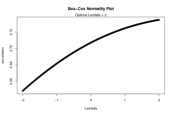
| Title produced by software | Box-Cox Normality Plot | ||||||||||||||||||||||||||||||||||||
| Date of computation | Mon, 05 Nov 2007 03:07:15 -0700 | ||||||||||||||||||||||||||||||||||||
| Cite this page as follows | Statistical Computations at FreeStatistics.org, Office for Research Development and Education, URL https://freestatistics.org/blog/index.php?v=date/2007/Nov/05/ry1rzv29sniz9bl1194257106.htm/, Retrieved Mon, 29 Apr 2024 04:52:10 +0000 | ||||||||||||||||||||||||||||||||||||
| Statistical Computations at FreeStatistics.org, Office for Research Development and Education, URL https://freestatistics.org/blog/index.php?pk=518, Retrieved Mon, 29 Apr 2024 04:52:10 +0000 | |||||||||||||||||||||||||||||||||||||
| QR Codes: | |||||||||||||||||||||||||||||||||||||
|
| |||||||||||||||||||||||||||||||||||||
| Original text written by user: | |||||||||||||||||||||||||||||||||||||
| IsPrivate? | No (this computation is public) | ||||||||||||||||||||||||||||||||||||
| User-defined keywords | Q4 | ||||||||||||||||||||||||||||||||||||
| Estimated Impact | 222 | ||||||||||||||||||||||||||||||||||||
Tree of Dependent Computations | |||||||||||||||||||||||||||||||||||||
| Family? (F = Feedback message, R = changed R code, M = changed R Module, P = changed Parameters, D = changed Data) | |||||||||||||||||||||||||||||||||||||
| - [Box-Cox Normality Plot] [Box cox normality...] [2007-11-05 10:07:15] [1329bc68d11d0852ec1dfd239c736a2c] [Current] F D [Box-Cox Normality Plot] [Various EDA Topic...] [2008-11-09 19:02:40] [57850c80fd59ccfb28f882be994e814e] | |||||||||||||||||||||||||||||||||||||
| Feedback Forum | |||||||||||||||||||||||||||||||||||||
Post a new message | |||||||||||||||||||||||||||||||||||||
Dataset | |||||||||||||||||||||||||||||||||||||
| Dataseries X: | |||||||||||||||||||||||||||||||||||||
12710,3 12120,8 12469,5 12054,6 12112,9 9617,2 12645,8 13581,3 12162,3 10969,7 11880,0 11887,6 12926,9 12300,0 12092,8 12380,8 12196,9 9455,0 13168,0 13427,9 11980,5 11884,8 11691,7 12233,8 14341,4 13130,7 12421,1 14285,8 12864,6 11160,2 14316,2 14388,7 14013,9 13419,0 12769,6 13315,5 15332,9 14243,0 13824,4 14962,9 13202,9 12199,0 15508,9 14199,8 15169,6 14058,0 13786,2 14147,9 16541,7 13587,5 15582,4 15802,8 14130,5 12923,2 15612,2 16033,7 16036,6 14037,8 15330,6 15038,3 17401,8 | |||||||||||||||||||||||||||||||||||||
Tables (Output of Computation) | |||||||||||||||||||||||||||||||||||||
| |||||||||||||||||||||||||||||||||||||
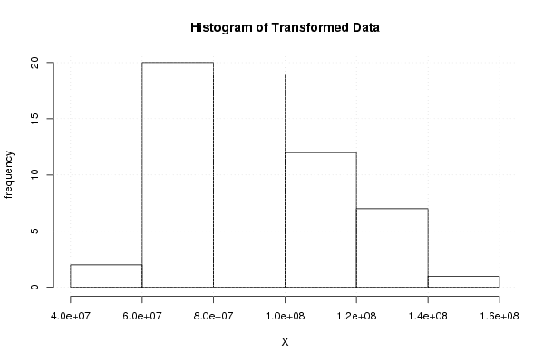
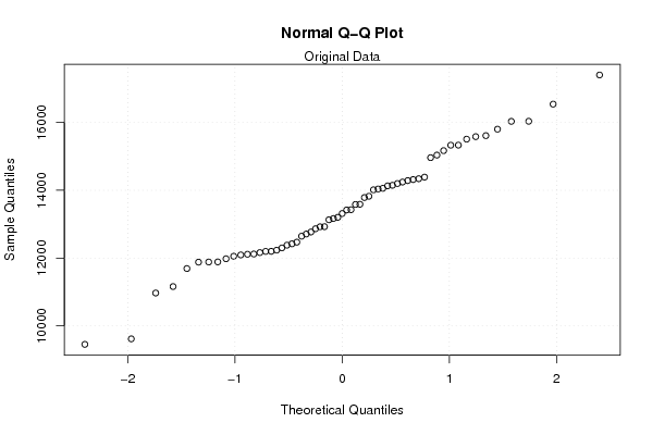
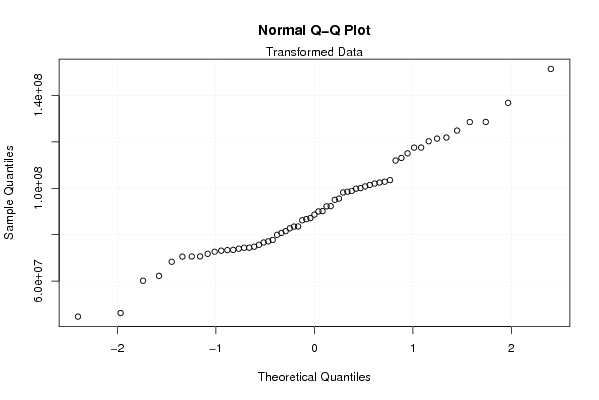
Figures (Output of Computation) | |||||||||||||||||||||||||||||||||||||
Input Parameters & R Code | |||||||||||||||||||||||||||||||||||||
| Parameters (Session): | |||||||||||||||||||||||||||||||||||||
| Parameters (R input): | |||||||||||||||||||||||||||||||||||||
| R code (references can be found in the software module): | |||||||||||||||||||||||||||||||||||||
n <- length(x) | |||||||||||||||||||||||||||||||||||||