Free Statistics
of Irreproducible Research!
Description of Statistical Computation | ||||||||||||||||||||||||||||||||||||||||||||||||
|---|---|---|---|---|---|---|---|---|---|---|---|---|---|---|---|---|---|---|---|---|---|---|---|---|---|---|---|---|---|---|---|---|---|---|---|---|---|---|---|---|---|---|---|---|---|---|---|---|
| Author's title | ||||||||||||||||||||||||||||||||||||||||||||||||
| Author | *Unverified author* | |||||||||||||||||||||||||||||||||||||||||||||||
| R Software Module | rwasp_fitdistrnorm.wasp | |||||||||||||||||||||||||||||||||||||||||||||||
| Title produced by software | ML Fitting and QQ Plot- Normal Distribution | |||||||||||||||||||||||||||||||||||||||||||||||
| Date of computation | Sat, 06 Feb 2021 22:15:44 +0100 | |||||||||||||||||||||||||||||||||||||||||||||||
| Cite this page as follows | Statistical Computations at FreeStatistics.org, Office for Research Development and Education, URL https://freestatistics.org/blog/index.php?v=date/2021/Feb/06/t16126462631ip2zjzw3rptewl.htm/, Retrieved Sat, 30 May 2026 17:07:45 +0000 | |||||||||||||||||||||||||||||||||||||||||||||||
| Statistical Computations at FreeStatistics.org, Office for Research Development and Education, URL https://freestatistics.org/blog/index.php?pk=319366, Retrieved Sat, 30 May 2026 17:07:45 +0000 | ||||||||||||||||||||||||||||||||||||||||||||||||
| QR Codes: | ||||||||||||||||||||||||||||||||||||||||||||||||
|
| ||||||||||||||||||||||||||||||||||||||||||||||||
| Original text written by user: | ||||||||||||||||||||||||||||||||||||||||||||||||
| IsPrivate? | No (this computation is public) | |||||||||||||||||||||||||||||||||||||||||||||||
| User-defined keywords | ||||||||||||||||||||||||||||||||||||||||||||||||
| Estimated Impact | 444 | |||||||||||||||||||||||||||||||||||||||||||||||
Tree of Dependent Computations | ||||||||||||||||||||||||||||||||||||||||||||||||
| Family? (F = Feedback message, R = changed R code, M = changed R Module, P = changed Parameters, D = changed Data) | ||||||||||||||||||||||||||||||||||||||||||||||||
| - [ML Fitting and QQ Plot- Normal Distribution] [] [2021-02-06 21:15:44] [d41d8cd98f00b204e9800998ecf8427e] [Current] | ||||||||||||||||||||||||||||||||||||||||||||||||
| Feedback Forum | ||||||||||||||||||||||||||||||||||||||||||||||||
Post a new message | ||||||||||||||||||||||||||||||||||||||||||||||||
Dataset | ||||||||||||||||||||||||||||||||||||||||||||||||
| Dataseries X: | ||||||||||||||||||||||||||||||||||||||||||||||||
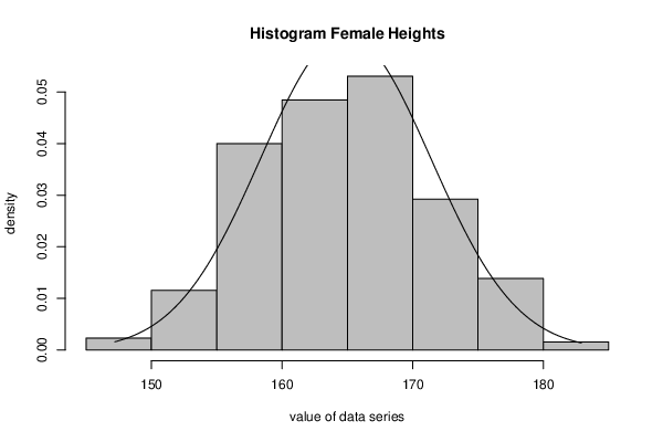
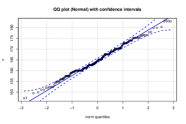
147.2 149.5 149.9 151.1 151.1 152.0 152.0 152.4 152.4 152.4 152.4 153.4 154.4 154.5 154.9 154.9 155.0 155.0 155.8 156.0 156.0 156.0 156.2 156.2 156.5 157.0 157.0 157.5 157.5 157.5 157.5 157.5 157.5 157.5 157.5 158.0 158.2 158.8 158.8 159.0 159.0 159.1 159.2 159.4 159.4 159.5 159.5 159.5 159.8 159.8 160.0 160.0 160.0 160.0 160.0 160.0 160.0 160.0 160.0 160.0 160.0 160.0 160.0 160.0 160.0 160.0 160.0 160.0 160.0 160.0 160.2 160.2 160.7 160.7 160.7 160.9 161.0 161.0 161.2 161.2 161.2 161.3 161.3 161.3 161.3 161.3 161.3 161.3 161.4 162.0 162.0 162.1 162.1 162.2 162.5 162.5 162.6 162.6 162.6 162.6 162.6 162.6 162.6 162.6 162.6 162.6 162.6 162.6 162.6 162.6 162.8 162.8 162.9 163.0 163.0 163.2 163.2 163.2 163.2 163.5 163.5 163.8 163.8 163.8 164.0 164.0 164.1 164.3 164.4 164.5 164.5 164.5 165.0 165.1 165.1 165.1 165.1 165.1 165.1 165.1 165.1 165.1 165.1 165.1 165.1 165.1 165.1 165.5 165.7 166.0 166.0 166.2 166.4 166.4 166.4 166.8 166.8 167.0 167.1 167.5 167.6 167.6 167.6 167.6 167.6 167.6 167.6 167.6 167.6 167.6 167.6 167.6 167.6 167.6 167.6 167.6 167.6 167.8 168.2 168.2 168.3 168.5 168.9 168.9 168.9 168.9 168.9 168.9 168.9 168.9 169.0 169.0 169.4 169.5 169.5 169.5 170.0 170.0 170.0 170.0 170.0 170.0 170.2 170.2 170.2 170.2 170.2 170.2 170.2 170.2 170.2 170.2 170.3 170.5 170.5 170.9 171.4 171.8 172.1 172.5 172.7 172.7 172.7 172.7 172.7 172.7 172.7 172.9 173.0 173.2 173.2 173.4 174.0 174.0 174.0 174.0 174.0 174.0 175.0 175.0 175.2 175.2 175.2 175.3 175.3 175.3 175.3 175.3 176.2 176.2 176.5 176.5 176.5 176.5 177.8 178.0 179.8 179.9 180.3 182.9 | ||||||||||||||||||||||||||||||||||||||||||||||||
Tables (Output of Computation) | ||||||||||||||||||||||||||||||||||||||||||||||||
| ||||||||||||||||||||||||||||||||||||||||||||||||
Figures (Output of Computation) | ||||||||||||||||||||||||||||||||||||||||||||||||
Input Parameters & R Code | ||||||||||||||||||||||||||||||||||||||||||||||||
| Parameters (Session): | ||||||||||||||||||||||||||||||||||||||||||||||||
| par1 = 8 ; par2 = 0 ; | ||||||||||||||||||||||||||||||||||||||||||||||||
| Parameters (R input): | ||||||||||||||||||||||||||||||||||||||||||||||||
| par1 = 8 ; par2 = 0 ; | ||||||||||||||||||||||||||||||||||||||||||||||||
| R code (references can be found in the software module): | ||||||||||||||||||||||||||||||||||||||||||||||||
par2 <- '0' | ||||||||||||||||||||||||||||||||||||||||||||||||