x <- c(1999.38
,1999.39
,1999.41
,1999.42
,1999.44
,1999.45
,1999.46
,1999.47
,1999.49
,1999.5
,1999.51
,1999.52
,1999.53
,1999.54
,1999.54
,1999.58
,1999.6
,1999.64
,1999.66
,1999.59
,1999.67
,1999.68
,1999.69
,1999.71
,1999.72
,1999.73
,1999.74
,1999.76
,1999.77
,1999.78
,1999.79
,1999.81
,1999.82
,1999.84
,1999.84
,1999.86
,1999.88
,1999.89
,1999.91
,1999.92
,1999.94
,1999.95
,1999.96
,1999.98
,2000
,2000.02
,2000.03
,2000.04
,2000.05
,2000.16
,2000.17
,2000.19
,2000.21
,2000.21
,2000.24
,2000.25
,2000.26
,2000.27
,2000.28
,2000.29
,2000.31
,2000.34
,2000.36
,2000.36
,2000.39
,2000.4
,2000.42
,2000.43
,2000.45
,2000.46
,2000.47
,2000.51
,2000.54
,2000.56
,2000.57
,2000.59
,2000.62
,2000.63
,2000.67
,2000.67
,2000.68
,2000.7
,2000.71
,2000.73
,2000.74
,2000.76
,2000.77
,2000.78
,2000.8
,2000.81
,2000.83
,2000.84
,2000.86
,2000.87
,2000.88
,2000.88
,2000.9
,2000.91
,2000.92
,2000.93
,2000.94
,2000.96
,2000.97
,2000.98
,2001.01
,2001.03
,2001.04
,2001.06
,2001.07
,2001.08
,2001.09
,2001.12
,2001.13
,2001.16
,2001.19
,2001.2
,2001.21
,2001.23
,2001.24
,2001.26
,2001.26
,2001.27
,2001.3
,2001.31
,2001.33
,2001.34
,2001.36
,2001.36
,2001.38
,2001.4
,2001.41
,2001.43
,2001.45
,2001.46
,2001.48
,2001.5
,2001.51
,2001.53
,2001.55
,2001.57
,2001.58
,2001.59
,2001.61
,2001.62
,2001.67
,2001.69
,2001.72
,2001.73
,2001.74
,2001.76
,2001.77
,2001.78
,2001.8
,2001.81
,2001.82
,2001.84
,2001.89
,2001.9
,2001.91
,2001.92
,2001.94
,2001.96
,2001.98
,2002.01
,2002.02
,2002.04
,2002.06
,2002.07
,2002.09
,2002.1
,2002.12
,2002.14
,2002.15
,2002.16
,2002.17
,2002.19
,2002.2
,2002.21
,2002.24
,2002.24
,2002.27
,2002.28
,2002.29
,2002.31
,2002.35
,2002.37
,2002.4
,2002.34
,2002.44
,2002.5
,2002.56
,2002.6
,2002.64
,2002.65
,2002.67
,2002.69
,2002.7
,2002.72
,2002.72
,2002.74
,2002.76
,2002.77
,2002.78
,2002.8
,2002.82
,2002.84
,2002.84
,2002.87
,2002.89
,2002.9
,2002.91
,2002.92
,2002.93
,2002.99
,2003.01
,2003.04
,2003.05
,2003.07
,2003.08
,2003.1
,2003.13
,2003.15
,2003.18
,2003.19
,2003.2
,2003.22
,2003.23
,2003.24
,2003.25
,2003.26
,2003.27
,2003.29
,2003.3
,2003.32
,2003.33
,2003.34
,2003.36
,2003.36
,2003.37
,2003.39
,2003.41
,2003.42
,2003.43
,2003.46
,2003.47
,2003.48
,2003.49
,2003.51
,2003.54
,2003.55
,2003.56
,2003.58
,2003.61
,2003.66
,2003.68
,2003.68
,2003.7
,2003.72
,2003.73
,2003.74
,2003.76
,2003.81
,2003.82
,2003.84
,2003.85
,2003.86
,2003.88
,2003.88
,2003.89
,2003.91
,2003.92
,2003.94
,2003.95
,2003.96
,2003.99
,2004.02
,2004.05
,2004.03
,2004.07
,2004.08
,2004.09
,2004.11
,2004.15
,2004.17
,2004.19
,2004.21
,2004.24
,2004.26
,2004.27
,2004.28
,2004.3
,2004.31
,2004.33
,2004.34
,2004.36
,2004.38
,2004.39
,2004.41
,2004.43
,2004.44
,2004.46
,2004.48)
y <- c(10.69
,9.09
,11.29
,10.59
,9.97
,9.65
,9.18
,10.49
,9.27
,10.4
,8.9
,9.17
,10.4
,9.53
,8.19
,10.04
,9.37
,10.46
,10.09
,7.38
,10.56
,9.83
,9.57
,10.46
,12.2
,7.64
,10.26
,9.43
,9.94
,11.19
,10.17
,9.61
,10.28
,12.06
,9.73
,10.1
,10.63
,10.64
,11.24
,9.4
,11.78
,9.75
,12.3
,11.35
,10.97
,11.77
,11.09
,11.43
,10.92
,11.91
,11.17
,10.04
,10.32
,9.6
,9.56
,10.27
,8.69
,10.91
,9.64
,9.09
,10.39
,10.15
,10.2
,9.28
,10.66
,9.37
,10.14
,10.43
,10.24
,9.28
,10.38
,9.85
,10.81
,12.2
,9.47
,9.49
,8.9
,9.76
,9.62
,9.6
,9.99
,10.48
,9.56
,9.19
,9.94
,9.57
,10.4
,9.26
,10.69
,10.35
,10
,9.34
,10.45
,10.76
,9.74
,7.34
,11.21
,10.67
,9.22
,10.34
,10.66
,9.96
,12.11
,10.71
,10.09
,10.25
,9.96
,11.73
,9.71
,10.1
,10.29
,11.05
,10.35
,12
,10.56
,10.43
,8.19
,11.38
,9.95
,10.51
,8.61
,10.29
,10.11
,10.12
,9.84
,10.05
,10.13
,9.97
,10.13
,9.87
,9.92
,9.44
,9.71
,9.77
,9.82
,10.31
,8.82
,9.62
,9.64
,10.69
,9.08
,9.59
,9.57
,8.17
,9.99
,9.09
,9.66
,9.21
,9.44
,10.04
,9.3
,10.24
,10.15
,10.2
,11.36
,9.5
,9.96
,10.15
,11.02
,10.05
,10.65
,10.31
,11.42
,10.08
,10.44
,10.39
,10.74
,10.99
,11.02
,10.55
,10.72
,10.54
,10.67
,10.35
,9.68
,10.78
,9.8
,11.09
,10.45
,10.66
,10.65
,9.9
,9.55
,9.91
,10.26
,10.14
,9.82
,10.27
,10.12
,9.52
,9.05
,10.26
,9.4
,8.99
,8.98
,9.49
,10.42
,9.31
,9.13
,9.71
,10.3
,9.75
,9.05
,10.91
,10.09
,11.15
,10.69
,10.36
,10.56
,10.52
,10.32
,9.78
,12.11
,10.75
,11.12
,10.32
,12.33
,10.03
,11.4
,12.47
,13.57
,10.2
,10.2
,10.84
,9.61
,10.35
,10
,9.76
,10.3
,9.86
,10.52
,10.49
,10.14
,10.11
,6.86
,9.58
,10.17
,8.9
,10.54
,9.49
,10.23
,9.04
,10.47
,11.88
,10.55
,8.86
,11.71
,9.88
,9.07
,9.63
,10.5
,10.16
,7.65
,8.56
,10.51
,8.9
,9.7
,9.83
,9.73
,9.03
,10.18
,9.45
,11.27
,10.35
,10.76
,11.2
,11.08
,9.17
,12.67
,11.09
,10.32
,10.71
,10.88
,8.44
,10.15
,10.06
,9.76
,12.45
,10.02
,8.89
,10.66
,10.71
,10.52
,10.58
,10.15
,11.1
,9.96
,11.31
,9.51
,6.98
,10.55
,7.22
,10.16
,8.03
,9.77
,10.36
,9.63
,10.6
,9.6
,8.75
,10.32
,10.23)
merc.df <- as.data.frame(cbind(x,y))
colnames(merc.df) <- c('date1','lp100km')
span <- as.numeric(par1)
if (par2 == 'TRUE') smooth <- TRUE else smooth <- FALSE
x=merc.df$date1
y=merc.df$lp100km
yl=loess(y~x,span=span)
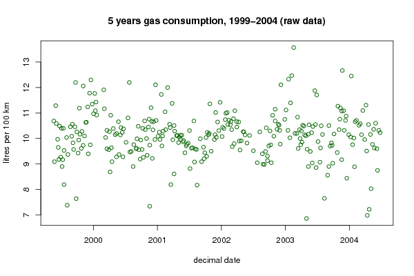
bitmap(file='noloessplot.png')
plot(yl,col='darkgreen',type='p',main='5 years gas consumption, 1999-2004 (raw data)',xlab='decimal date',ylab='litres per 100 km')
dev.off()
if (smooth==TRUE)
{
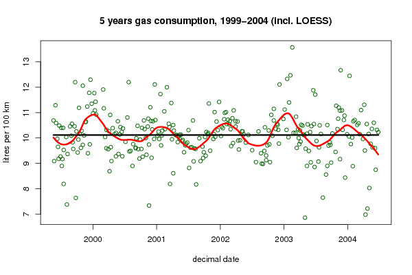
bitmap(file='loessplot.png')
plot(yl,col='darkgreen',type='p',main='5 years gas consumption, 1999-2004 (incl. LOESS)',xlab='decimal date',ylab='litres per 100 km')
mn=mean(yl$y)
lines(yl$x,yl$fitted,col='red',lwd=3)
lines(yl$x,mn*rep(1,length(yl$x)),col='black',lwd=3)
dev.off()
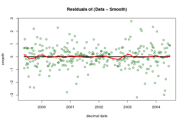
bitmap(file='resplot.png')
plot(yl$x,yl$residuals,col='darkgreen',ylab='residuals from
smooth',xlab='decimal date',main='Residuals of (Data - Smooth)')
lines(yl$x,0*rep(1,length(yl$x)),col='black',lwd=3)
rl=loess(yl$residuals~yl$x,span=span)
lines(rl$x,rl$fitted,col='red',lwd=3)
dev.off()
}
|