require('stsm')
require('stsm.class')
require('KFKSDS')
par1 <- as.numeric(par1)
par2 <- as.numeric(par2)
nx <- length(x)
x <- ts(x,frequency=par1)
m <- StructTS(x,type='BSM')
print(m$coef)
print(m$fitted)
print(m$resid)
mylevel <- as.numeric(m$fitted[,'level'])
myslope <- as.numeric(m$fitted[,'slope'])
myseas <- as.numeric(m$fitted[,'sea'])
myresid <- as.numeric(m$resid)
myfit <- mylevel+myseas
mm <- stsm.model(model = 'BSM', y = x, transPars = 'StructTS')
fit2 <- stsmFit(mm, stsm.method = 'maxlik.td.optim', method = par3, KF.args = list(P0cov = TRUE))
(fit2.comps <- tsSmooth(fit2, P0cov = FALSE)$states)
m2 <- set.pars(mm, pmax(fit2$par, .Machine$double.eps))
(ss <- char2numeric(m2))
(pred <- predict(ss, x, n.ahead = par2))
mylagmax <- nx/2
bitmap(file='test2.png')
op <- par(mfrow = c(2,2))
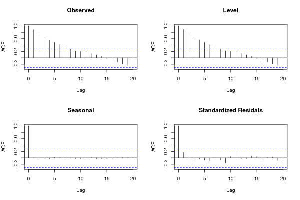
acf(as.numeric(x),lag.max = mylagmax,main='Observed')
acf(mylevel,na.action=na.pass,lag.max = mylagmax,main='Level')
acf(myseas,na.action=na.pass,lag.max = mylagmax,main='Seasonal')
acf(myresid,na.action=na.pass,lag.max = mylagmax,main='Standardized Residals')
par(op)
dev.off()
bitmap(file='test3.png')
op <- par(mfrow = c(2,2))
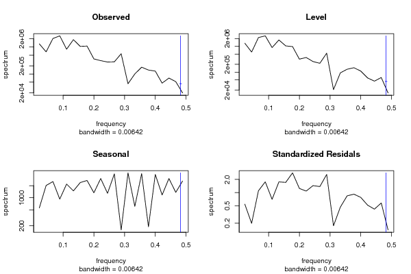
spectrum(as.numeric(x),main='Observed')
spectrum(mylevel,main='Level')
spectrum(myseas,main='Seasonal')
spectrum(myresid,main='Standardized Residals')
par(op)
dev.off()
bitmap(file='test4.png')
op <- par(mfrow = c(2,2))
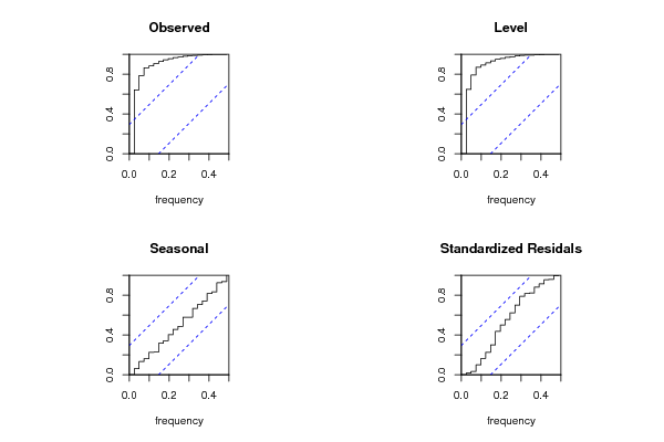
cpgram(as.numeric(x),main='Observed')
cpgram(mylevel,main='Level')
cpgram(myseas,main='Seasonal')
cpgram(myresid,main='Standardized Residals')
par(op)
dev.off()
bitmap(file='test1.png')
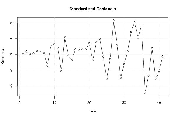
plot(as.numeric(m$resid),main='Standardized Residuals',ylab='Residuals',xlab='time',type='b')
grid()
dev.off()
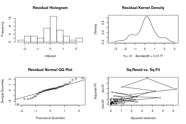
bitmap(file='test5.png')
op <- par(mfrow = c(2,2))
hist(m$resid,main='Residual Histogram')
plot(density(m$resid),main='Residual Kernel Density')
qqnorm(m$resid,main='Residual Normal QQ Plot')
qqline(m$resid)
plot(m$resid^2, myfit^2,main='Sq.Resid vs. Sq.Fit',xlab='Squared residuals',ylab='Squared Fit')
par(op)
dev.off()
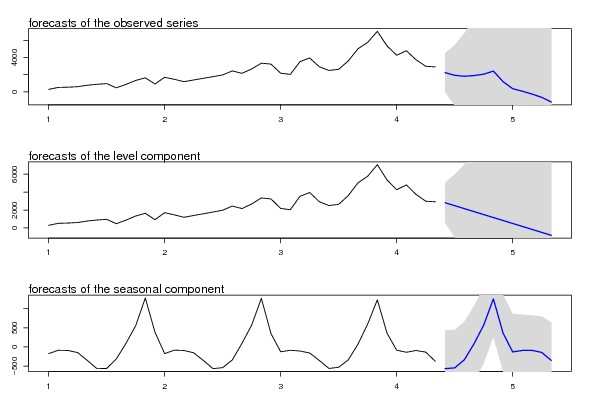
bitmap(file='test6.png')
par(mfrow = c(3,1), mar = c(3,3,3,3))
plot(cbind(x, pred$pred), type = 'n', plot.type = 'single', ylab = '')
lines(x)
polygon(c(time(pred$pred), rev(time(pred$pred))), c(pred$pred + 2 * pred$se, rev(pred$pred)), col = 'gray85', border = NA)
polygon(c(time(pred$pred), rev(time(pred$pred))), c(pred$pred - 2 * pred$se, rev(pred$pred)), col = ' gray85', border = NA)
lines(pred$pred, col = 'blue', lwd = 1.5)
mtext(text = 'forecasts of the observed series', side = 3, adj = 0)
plot(cbind(x, pred$a[,1]), type = 'n', plot.type = 'single', ylab = '')
lines(x)
polygon(c(time(pred$a[,1]), rev(time(pred$a[,1]))), c(pred$a[,1] + 2 * sqrt(pred$P[,1]), rev(pred$a[,1])), col = 'gray85', border = NA)
polygon(c(time(pred$a[,1]), rev(time(pred$a[,1]))), c(pred$a[,1] - 2 * sqrt(pred$P[,1]), rev(pred$a[,1])), col = ' gray85', border = NA)
lines(pred$a[,1], col = 'blue', lwd = 1.5)
mtext(text = 'forecasts of the level component', side = 3, adj = 0)
plot(cbind(fit2.comps[,3], pred$a[,3]), type = 'n', plot.type = 'single', ylab = '')
lines(fit2.comps[,3])
polygon(c(time(pred$a[,3]), rev(time(pred$a[,3]))), c(pred$a[,3] + 2 * sqrt(pred$P[,3]), rev(pred$a[,3])), col = 'gray85', border = NA)
polygon(c(time(pred$a[,3]), rev(time(pred$a[,3]))), c(pred$a[,3] - 2 * sqrt(pred$P[,3]), rev(pred$a[,3])), col = ' gray85', border = NA)
lines(pred$a[,3], col = 'blue', lwd = 1.5)
mtext(text = 'forecasts of the seasonal component', side = 3, adj = 0)
dev.off()
load(file='createtable')
a<-table.start()
a<-table.row.start(a)
a<-table.element(a,'Structural Time Series Model -- Interpolation',6,TRUE)
a<-table.row.end(a)
a<-table.row.start(a)
a<-table.element(a,'t',header=TRUE)
a<-table.element(a,'Observed',header=TRUE)
a<-table.element(a,'Level',header=TRUE)
a<-table.element(a,'Slope',header=TRUE)
a<-table.element(a,'Seasonal',header=TRUE)
a<-table.element(a,'Stand. Residuals',header=TRUE)
a<-table.row.end(a)
for (i in 1:nx) {
a<-table.row.start(a)
a<-table.element(a,i,header=TRUE)
a<-table.element(a,x[i])
a<-table.element(a,mylevel[i])
a<-table.element(a,myslope[i])
a<-table.element(a,myseas[i])
a<-table.element(a,myresid[i])
a<-table.row.end(a)
}
a<-table.end(a)
table.save(a,file='mytable.tab')
a<-table.start()
a<-table.row.start(a)
a<-table.element(a,'Structural Time Series Model -- Extrapolation',4,TRUE)
a<-table.row.end(a)
a<-table.row.start(a)
a<-table.element(a,'t',header=TRUE)
a<-table.element(a,'Observed',header=TRUE)
a<-table.element(a,'Level',header=TRUE)
a<-table.element(a,'Seasonal',header=TRUE)
a<-table.row.end(a)
for (i in 1:par2) {
a<-table.row.start(a)
a<-table.element(a,i,header=TRUE)
a<-table.element(a,pred$pred[i])
a<-table.element(a,pred$a[i,1])
a<-table.element(a,pred$a[i,3])
a<-table.row.end(a)
}
a<-table.end(a)
table.save(a,file='mytable1.tab')
|