Repository of Reproducible Computations

Free Statistics

of Irreproducible Research!

Author's title

Author

*Unverified author*

R Software Module

rwasp_histogram.wasp

Title produced by software

Histogram

Date of computation

Thu, 20 Feb 2014 04:40:05 -0500

Cite this page as follows

Statistical Computations at FreeStatistics.org, Office for Research Development and Education, URL https://freestatistics.org/blog/index.php?v=date/2014/Feb/20/t1392889409wuff8f8ue0e39lq.htm/, Retrieved Wed, 15 May 2024 06:04:56 +0000

Statistical Computations at FreeStatistics.org, Office for Research Development and Education, URL https://freestatistics.org/blog/index.php?pk=233906, Retrieved Wed, 15 May 2024 06:04:56 +0000

QR Codes:

Paste this QR Code to cite your computation.

Original text written by user:

Numerische Mathematik I (Mathe BSc) (B�rwolff/Kandler) http://www3.math.tu-berlin.de/Vorlesungen/WS13/NumMath1/ Punktestand vor Einsicht. max 40 P., bestanden = 21 P. Durchfallquote 43,75% !

IsPrivate?

No (this computation is public)

User-defined keywords

Estimated Impact

140

Family? (F = Feedback message, R = changed R code, M = changed R Module, P = changed Parameters, D = changed Data)

-     [Histogram] [tu berlin lina1 k...] [2012-07-11 21:49:14] [74be16979710d4c4e7c6647856088456]
- R  D  [Histogram] [Ergebnisse Modulk...] [2013-09-24 18:06:22] [74be16979710d4c4e7c6647856088456]
-   PD    [Histogram] [TU WS2013/14 Nume...] [2014-02-20 09:07:22] [74be16979710d4c4e7c6647856088456]
-   PD      [Histogram] [NumMath1-Modulkla...] [2014-02-20 09:28:44] [74be16979710d4c4e7c6647856088456]
-               [Histogram] [NumMath1-Modulkla...] [2014-02-20 09:40:05] [d41d8cd98f00b204e9800998ecf8427e] [Current]
-    D            [Histogram] [NumMath1-Modulkla...] [2014-04-04 15:20:24] [74be16979710d4c4e7c6647856088456] 
-    D              [Histogram] [Noten Juli-Klausu...] [2014-07-24 02:44:35] [74be16979710d4c4e7c6647856088456] 

Feedback Forum

Post a new message

Dataseries X:

Download CSV

Histogram

Boxplots

Summary of computational transaction
Raw Input	view raw input (R code)
Raw Output	view raw output of R engine
Computing time	3 seconds
R Server	'Herman Ole Andreas Wold' @ wold.wessa.net

\begin{tabular}{lllllllll}
\hline
Summary of computational transaction \tabularnewline
Raw Input & view raw input (R code)  \tabularnewline
Raw Output & view raw output of R engine  \tabularnewline
Computing time & 3 seconds \tabularnewline
R Server & 'Herman Ole Andreas Wold' @ wold.wessa.net \tabularnewline
\hline
\end{tabular}
%Source: https://freestatistics.org/blog/index.php?pk=233906&T=0

[TABLE]
[ROW][C]Summary of computational transaction[/C][/ROW]
[ROW][C]Raw Input[/C][C]view raw input (R code) [/C][/ROW]
[ROW][C]Raw Output[/C][C]view raw output of R engine [/C][/ROW]
[ROW][C]Computing time[/C][C]3 seconds[/C][/ROW]
[ROW][C]R Server[/C][C]'Herman Ole Andreas Wold' @ wold.wessa.net[/C][/ROW]
[/TABLE]
Source: https://freestatistics.org/blog/index.php?pk=233906&T=0

Globally Unique Identifier (entire table): ba.freestatistics.org/blog/index.php?pk=233906&T=0

As an alternative you can also use a QR Code:

The GUIDs for individual cells are displayed in the table below:

Summary of computational transaction
Raw Input	view raw input (R code)
Raw Output	view raw output of R engine
Computing time	3 seconds
R Server	'Herman Ole Andreas Wold' @ wold.wessa.net

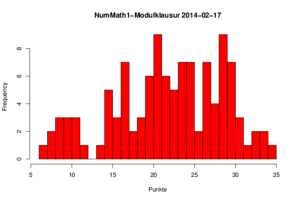
Frequency Table (Histogram)
Bins	Midpoint	Abs. Frequency	Rel. Frequency	Cumul. Rel. Freq.	Density
[6,7[	6.5	1	0.008929	0.008929	0.008929
[7,8[	7.5	2	0.017857	0.026786	0.017857
[8,9[	8.5	3	0.026786	0.053571	0.026786
[9,10[	9.5	3	0.026786	0.080357	0.026786
[10,11[	10.5	3	0.026786	0.107143	0.026786
[11,12[	11.5	1	0.008929	0.116071	0.008929
[12,13[	12.5	0	0	0.116071	0
[13,14[	13.5	1	0.008929	0.125	0.008929
[14,15[	14.5	5	0.044643	0.169643	0.044643
[15,16[	15.5	3	0.026786	0.196429	0.026786
[16,17[	16.5	7	0.0625	0.258929	0.0625
[17,18[	17.5	2	0.017857	0.276786	0.017857
[18,19[	18.5	3	0.026786	0.303571	0.026786
[19,20[	19.5	6	0.053571	0.357143	0.053571
[20,21[	20.5	9	0.080357	0.4375	0.080357
[21,22[	21.5	6	0.053571	0.491071	0.053571
[22,23[	22.5	5	0.044643	0.535714	0.044643
[23,24[	23.5	7	0.0625	0.598214	0.0625
[24,25[	24.5	7	0.0625	0.660714	0.0625
[25,26[	25.5	2	0.017857	0.678571	0.017857
[26,27[	26.5	7	0.0625	0.741071	0.0625
[27,28[	27.5	4	0.035714	0.776786	0.035714
[28,29[	28.5	9	0.080357	0.857143	0.080357
[29,30[	29.5	7	0.0625	0.919643	0.0625
[30,31[	30.5	3	0.026786	0.946429	0.026786
[31,32[	31.5	1	0.008929	0.955357	0.008929
[32,33[	32.5	2	0.017857	0.973214	0.017857
[33,34[	33.5	2	0.017857	0.991071	0.017857
[34,35]	34.5	1	0.008929	1	0.008929

\begin{tabular}{lllllllll}
\hline
Frequency Table (Histogram) \tabularnewline
Bins & Midpoint & Abs. Frequency & Rel. Frequency & Cumul. Rel. Freq. & Density \tabularnewline
[6,7[ & 6.5 & 1 & 0.008929 & 0.008929 & 0.008929 \tabularnewline
[7,8[ & 7.5 & 2 & 0.017857 & 0.026786 & 0.017857 \tabularnewline
[8,9[ & 8.5 & 3 & 0.026786 & 0.053571 & 0.026786 \tabularnewline
[9,10[ & 9.5 & 3 & 0.026786 & 0.080357 & 0.026786 \tabularnewline
[10,11[ & 10.5 & 3 & 0.026786 & 0.107143 & 0.026786 \tabularnewline
[11,12[ & 11.5 & 1 & 0.008929 & 0.116071 & 0.008929 \tabularnewline
[12,13[ & 12.5 & 0 & 0 & 0.116071 & 0 \tabularnewline
[13,14[ & 13.5 & 1 & 0.008929 & 0.125 & 0.008929 \tabularnewline
[14,15[ & 14.5 & 5 & 0.044643 & 0.169643 & 0.044643 \tabularnewline
[15,16[ & 15.5 & 3 & 0.026786 & 0.196429 & 0.026786 \tabularnewline
[16,17[ & 16.5 & 7 & 0.0625 & 0.258929 & 0.0625 \tabularnewline
[17,18[ & 17.5 & 2 & 0.017857 & 0.276786 & 0.017857 \tabularnewline
[18,19[ & 18.5 & 3 & 0.026786 & 0.303571 & 0.026786 \tabularnewline
[19,20[ & 19.5 & 6 & 0.053571 & 0.357143 & 0.053571 \tabularnewline
[20,21[ & 20.5 & 9 & 0.080357 & 0.4375 & 0.080357 \tabularnewline
[21,22[ & 21.5 & 6 & 0.053571 & 0.491071 & 0.053571 \tabularnewline
[22,23[ & 22.5 & 5 & 0.044643 & 0.535714 & 0.044643 \tabularnewline
[23,24[ & 23.5 & 7 & 0.0625 & 0.598214 & 0.0625 \tabularnewline
[24,25[ & 24.5 & 7 & 0.0625 & 0.660714 & 0.0625 \tabularnewline
[25,26[ & 25.5 & 2 & 0.017857 & 0.678571 & 0.017857 \tabularnewline
[26,27[ & 26.5 & 7 & 0.0625 & 0.741071 & 0.0625 \tabularnewline
[27,28[ & 27.5 & 4 & 0.035714 & 0.776786 & 0.035714 \tabularnewline
[28,29[ & 28.5 & 9 & 0.080357 & 0.857143 & 0.080357 \tabularnewline
[29,30[ & 29.5 & 7 & 0.0625 & 0.919643 & 0.0625 \tabularnewline
[30,31[ & 30.5 & 3 & 0.026786 & 0.946429 & 0.026786 \tabularnewline
[31,32[ & 31.5 & 1 & 0.008929 & 0.955357 & 0.008929 \tabularnewline
[32,33[ & 32.5 & 2 & 0.017857 & 0.973214 & 0.017857 \tabularnewline
[33,34[ & 33.5 & 2 & 0.017857 & 0.991071 & 0.017857 \tabularnewline
[34,35] & 34.5 & 1 & 0.008929 & 1 & 0.008929 \tabularnewline
\hline
\end{tabular}
%Source: https://freestatistics.org/blog/index.php?pk=233906&T=1

[TABLE]
[ROW][C]Frequency Table (Histogram)[/C][/ROW]
[ROW][C]Bins[/C][C]Midpoint[/C][C]Abs. Frequency[/C][C]Rel. Frequency[/C][C]Cumul. Rel. Freq.[/C][C]Density[/C][/ROW]
[ROW][C][6,7[[/C][C]6.5[/C][C]1[/C][C]0.008929[/C][C]0.008929[/C][C]0.008929[/C][/ROW]
[ROW][C][7,8[[/C][C]7.5[/C][C]2[/C][C]0.017857[/C][C]0.026786[/C][C]0.017857[/C][/ROW]
[ROW][C][8,9[[/C][C]8.5[/C][C]3[/C][C]0.026786[/C][C]0.053571[/C][C]0.026786[/C][/ROW]
[ROW][C][9,10[[/C][C]9.5[/C][C]3[/C][C]0.026786[/C][C]0.080357[/C][C]0.026786[/C][/ROW]
[ROW][C][10,11[[/C][C]10.5[/C][C]3[/C][C]0.026786[/C][C]0.107143[/C][C]0.026786[/C][/ROW]
[ROW][C][11,12[[/C][C]11.5[/C][C]1[/C][C]0.008929[/C][C]0.116071[/C][C]0.008929[/C][/ROW]
[ROW][C][12,13[[/C][C]12.5[/C][C]0[/C][C]0[/C][C]0.116071[/C][C]0[/C][/ROW]
[ROW][C][13,14[[/C][C]13.5[/C][C]1[/C][C]0.008929[/C][C]0.125[/C][C]0.008929[/C][/ROW]
[ROW][C][14,15[[/C][C]14.5[/C][C]5[/C][C]0.044643[/C][C]0.169643[/C][C]0.044643[/C][/ROW]
[ROW][C][15,16[[/C][C]15.5[/C][C]3[/C][C]0.026786[/C][C]0.196429[/C][C]0.026786[/C][/ROW]
[ROW][C][16,17[[/C][C]16.5[/C][C]7[/C][C]0.0625[/C][C]0.258929[/C][C]0.0625[/C][/ROW]
[ROW][C][17,18[[/C][C]17.5[/C][C]2[/C][C]0.017857[/C][C]0.276786[/C][C]0.017857[/C][/ROW]
[ROW][C][18,19[[/C][C]18.5[/C][C]3[/C][C]0.026786[/C][C]0.303571[/C][C]0.026786[/C][/ROW]
[ROW][C][19,20[[/C][C]19.5[/C][C]6[/C][C]0.053571[/C][C]0.357143[/C][C]0.053571[/C][/ROW]
[ROW][C][20,21[[/C][C]20.5[/C][C]9[/C][C]0.080357[/C][C]0.4375[/C][C]0.080357[/C][/ROW]
[ROW][C][21,22[[/C][C]21.5[/C][C]6[/C][C]0.053571[/C][C]0.491071[/C][C]0.053571[/C][/ROW]
[ROW][C][22,23[[/C][C]22.5[/C][C]5[/C][C]0.044643[/C][C]0.535714[/C][C]0.044643[/C][/ROW]
[ROW][C][23,24[[/C][C]23.5[/C][C]7[/C][C]0.0625[/C][C]0.598214[/C][C]0.0625[/C][/ROW]
[ROW][C][24,25[[/C][C]24.5[/C][C]7[/C][C]0.0625[/C][C]0.660714[/C][C]0.0625[/C][/ROW]
[ROW][C][25,26[[/C][C]25.5[/C][C]2[/C][C]0.017857[/C][C]0.678571[/C][C]0.017857[/C][/ROW]
[ROW][C][26,27[[/C][C]26.5[/C][C]7[/C][C]0.0625[/C][C]0.741071[/C][C]0.0625[/C][/ROW]
[ROW][C][27,28[[/C][C]27.5[/C][C]4[/C][C]0.035714[/C][C]0.776786[/C][C]0.035714[/C][/ROW]
[ROW][C][28,29[[/C][C]28.5[/C][C]9[/C][C]0.080357[/C][C]0.857143[/C][C]0.080357[/C][/ROW]
[ROW][C][29,30[[/C][C]29.5[/C][C]7[/C][C]0.0625[/C][C]0.919643[/C][C]0.0625[/C][/ROW]
[ROW][C][30,31[[/C][C]30.5[/C][C]3[/C][C]0.026786[/C][C]0.946429[/C][C]0.026786[/C][/ROW]
[ROW][C][31,32[[/C][C]31.5[/C][C]1[/C][C]0.008929[/C][C]0.955357[/C][C]0.008929[/C][/ROW]
[ROW][C][32,33[[/C][C]32.5[/C][C]2[/C][C]0.017857[/C][C]0.973214[/C][C]0.017857[/C][/ROW]
[ROW][C][33,34[[/C][C]33.5[/C][C]2[/C][C]0.017857[/C][C]0.991071[/C][C]0.017857[/C][/ROW]
[ROW][C][34,35][/C][C]34.5[/C][C]1[/C][C]0.008929[/C][C]1[/C][C]0.008929[/C][/ROW]
[/TABLE]
Source: https://freestatistics.org/blog/index.php?pk=233906&T=1

Globally Unique Identifier (entire table): ba.freestatistics.org/blog/index.php?pk=233906&T=1

As an alternative you can also use a QR Code:

The GUIDs for individual cells are displayed in the table below:

Frequency Table (Histogram)
Bins	Midpoint	Abs. Frequency	Rel. Frequency	Cumul. Rel. Freq.	Density
[6,7[	6.5	1	0.008929	0.008929	0.008929
[7,8[	7.5	2	0.017857	0.026786	0.017857
[8,9[	8.5	3	0.026786	0.053571	0.026786
[9,10[	9.5	3	0.026786	0.080357	0.026786
[10,11[	10.5	3	0.026786	0.107143	0.026786
[11,12[	11.5	1	0.008929	0.116071	0.008929
[12,13[	12.5	0	0	0.116071	0
[13,14[	13.5	1	0.008929	0.125	0.008929
[14,15[	14.5	5	0.044643	0.169643	0.044643
[15,16[	15.5	3	0.026786	0.196429	0.026786
[16,17[	16.5	7	0.0625	0.258929	0.0625
[17,18[	17.5	2	0.017857	0.276786	0.017857
[18,19[	18.5	3	0.026786	0.303571	0.026786
[19,20[	19.5	6	0.053571	0.357143	0.053571
[20,21[	20.5	9	0.080357	0.4375	0.080357
[21,22[	21.5	6	0.053571	0.491071	0.053571
[22,23[	22.5	5	0.044643	0.535714	0.044643
[23,24[	23.5	7	0.0625	0.598214	0.0625
[24,25[	24.5	7	0.0625	0.660714	0.0625
[25,26[	25.5	2	0.017857	0.678571	0.017857
[26,27[	26.5	7	0.0625	0.741071	0.0625
[27,28[	27.5	4	0.035714	0.776786	0.035714
[28,29[	28.5	9	0.080357	0.857143	0.080357
[29,30[	29.5	7	0.0625	0.919643	0.0625
[30,31[	30.5	3	0.026786	0.946429	0.026786
[31,32[	31.5	1	0.008929	0.955357	0.008929
[32,33[	32.5	2	0.017857	0.973214	0.017857
[33,34[	33.5	2	0.017857	0.991071	0.017857
[34,35]	34.5	1	0.008929	1	0.008929

Figure 1

PNG link

Postscript link

PDF link

Parameters (Session):

par1 = 30 ; par2 = red ; par3 = FALSE ; par4 = Unknown ;

Parameters (R input):

par1 = 30 ; par2 = red ; par3 = FALSE ; par4 = Unknown ;

R code (references can be found in the software module):

par1 <- as.numeric(par1)
if (par3 == 'TRUE') par3 <- TRUE
if (par3 == 'FALSE') par3 <- FALSE
if (par4 == 'Unknown') par1 <- as.numeric(par1)
if (par4 == 'Interval/Ratio') par1 <- as.numeric(par1)
if (par4 == '3-point Likert') par1 <- c(1:3 - 0.5, 3.5)
if (par4 == '4-point Likert') par1 <- c(1:4 - 0.5, 4.5)
if (par4 == '5-point Likert') par1 <- c(1:5 - 0.5, 5.5)
if (par4 == '6-point Likert') par1 <- c(1:6 - 0.5, 6.5)
if (par4 == '7-point Likert') par1 <- c(1:7 - 0.5, 7.5)
if (par4 == '8-point Likert') par1 <- c(1:8 - 0.5, 8.5)
if (par4 == '9-point Likert') par1 <- c(1:9 - 0.5, 9.5)
if (par4 == '10-point Likert') par1 <- c(1:10 - 0.5, 10.5)
bitmap(file='test1.png')
if(is.numeric(x[1])) {
if (is.na(par1)) {
myhist<-hist(x,col=par2,main=main,xlab=xlab,right=par3)
} else {
if (par1 < 0) par1 <- 3
if (par1 > 50) par1 <- 50
myhist<-hist(x,breaks=par1,col=par2,main=main,xlab=xlab,right=par3)
}
} else {
plot(mytab <- table(x),col=par2,main='Frequency Plot',xlab=xlab,ylab='Absolute Frequency')
}
dev.off()
if(is.numeric(x[1])) {
myhist
n <- length(x)
load(file='createtable')
a<-table.start()
a<-table.row.start(a)
a<-table.element(a,hyperlink('histogram.htm','Frequency Table (Histogram)',''),6,TRUE)
a<-table.row.end(a)
a<-table.row.start(a)
a<-table.element(a,'Bins',header=TRUE)
a<-table.element(a,'Midpoint',header=TRUE)
a<-table.element(a,'Abs. Frequency',header=TRUE)
a<-table.element(a,'Rel. Frequency',header=TRUE)
a<-table.element(a,'Cumul. Rel. Freq.',header=TRUE)
a<-table.element(a,'Density',header=TRUE)
a<-table.row.end(a)
crf <- 0
if (par3 == FALSE) mybracket <- '[' else mybracket <- ']'
mynumrows <- (length(myhist$breaks)-1)
for (i in 1:mynumrows) {
a<-table.row.start(a)
if (i == 1)
dum <- paste('[',myhist$breaks[i],sep='')
else
dum <- paste(mybracket,myhist$breaks[i],sep='')
dum <- paste(dum,myhist$breaks[i+1],sep=',')
if (i==mynumrows)
dum <- paste(dum,']',sep='')
else
dum <- paste(dum,mybracket,sep='')
a<-table.element(a,dum,header=TRUE)
a<-table.element(a,myhist$mids[i])
a<-table.element(a,myhist$counts[i])
rf <- myhist$counts[i]/n
crf <- crf + rf
a<-table.element(a,round(rf,6))
a<-table.element(a,round(crf,6))
a<-table.element(a,round(myhist$density[i],6))
a<-table.row.end(a)
}
a<-table.end(a)
table.save(a,file='mytable.tab')
} else {
mytab
reltab <- mytab / sum(mytab)
n <- length(mytab)
load(file='createtable')
a<-table.start()
a<-table.row.start(a)
a<-table.element(a,'Frequency Table (Categorical Data)',3,TRUE)
a<-table.row.end(a)
a<-table.row.start(a)
a<-table.element(a,'Category',header=TRUE)
a<-table.element(a,'Abs. Frequency',header=TRUE)
a<-table.element(a,'Rel. Frequency',header=TRUE)
a<-table.row.end(a)
for (i in 1:n) {
a<-table.row.start(a)
a<-table.element(a,labels(mytab)$x[i],header=TRUE)
a<-table.element(a,mytab[i])
a<-table.element(a,round(reltab[i],4))
a<-table.row.end(a)
}
a<-table.end(a)
table.save(a,file='mytable1.tab')
}

Free Statistics

Description of Statistical Computation

Tree of Dependent Computations

Dataset

Tables (Output of Computation)

Figures (Output of Computation)

Input Parameters & R Code