Repository of Reproducible Computations

Free Statistics

of Irreproducible Research!

Author's title

Author

*The author of this computation has been verified*

R Software Module

rwasp_autocorrelation.wasp

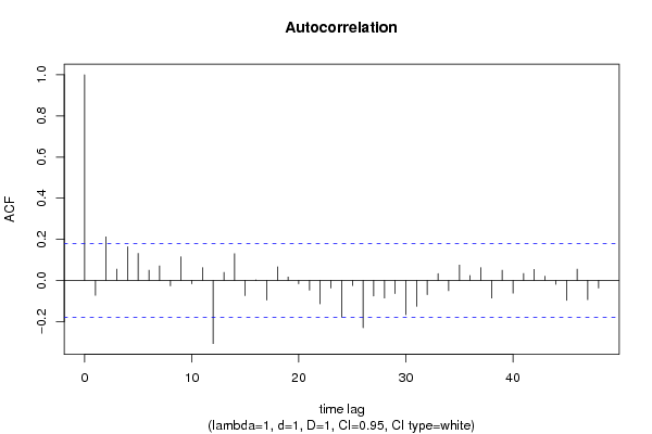
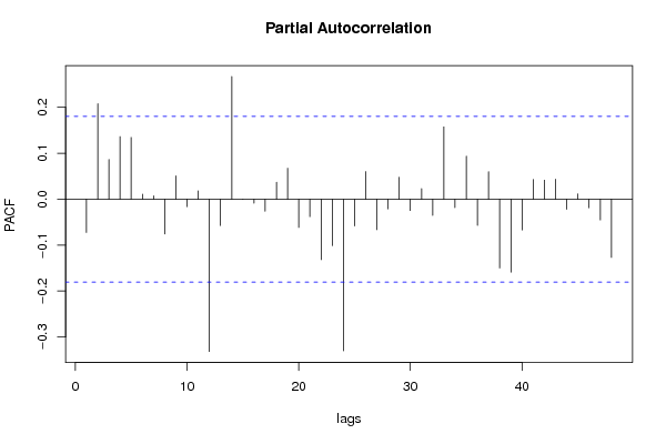
Title produced by software

(Partial) Autocorrelation Function

Date of computation

Tue, 21 Dec 2010 19:26:54 +0000

Cite this page as follows

Statistical Computations at FreeStatistics.org, Office for Research Development and Education, URL https://freestatistics.org/blog/index.php?v=date/2010/Dec/21/t1292959492kejho809li06o4q.htm/, Retrieved Thu, 16 May 2024 01:30:26 +0000

Statistical Computations at FreeStatistics.org, Office for Research Development and Education, URL https://freestatistics.org/blog/index.php?pk=113871, Retrieved Thu, 16 May 2024 01:30:26 +0000

QR Codes:

Paste this QR Code to cite your computation.

Original text written by user:

IsPrivate?

No (this computation is public)

User-defined keywords

Estimated Impact

170

Family? (F = Feedback message, R = changed R code, M = changed R Module, P = changed Parameters, D = changed Data)

-     [Variance Reduction Matrix] [Unemployment] [2010-11-29 09:29:57] [b98453cac15ba1066b407e146608df68]
-   PD  [Variance Reduction Matrix] [WS9 - Variance Re...] [2010-12-04 11:04:59] [8ef49741e164ec6343c90c7935194465]
-   P     [Variance Reduction Matrix] [WS 9 VRM] [2010-12-05 14:01:21] [8214fe6d084e5ad7598b249a26cc9f06]
- RMPD      [(Partial) Autocorrelation Function] [paper ACF] [2010-12-10 10:47:04] [8214fe6d084e5ad7598b249a26cc9f06]
-   P         [(Partial) Autocorrelation Function] [paper acf met D=1] [2010-12-10 11:19:24] [8214fe6d084e5ad7598b249a26cc9f06]
-   PD          [(Partial) Autocorrelation Function] [acf 2] [2010-12-20 19:51:16] [8214fe6d084e5ad7598b249a26cc9f06]
-   PD              [(Partial) Autocorrelation Function] [acf 2 laaggeschoo...] [2010-12-21 19:26:54] [b47314d83d48c7bf812ec2bcd743b159] [Current]

Feedback Forum

Post a new message

Dataseries X:

Download CSV

Histogram

Boxplots

Summary of computational transaction
Raw Input	view raw input (R code)
Raw Output	view raw output of R engine
Computing time	1 seconds
R Server	'Gwilym Jenkins' @ 72.249.127.135

\begin{tabular}{lllllllll}
\hline
Summary of computational transaction \tabularnewline
Raw Input & view raw input (R code)  \tabularnewline
Raw Output & view raw output of R engine  \tabularnewline
Computing time & 1 seconds \tabularnewline
R Server & 'Gwilym Jenkins' @ 72.249.127.135 \tabularnewline
\hline
\end{tabular}
%Source: https://freestatistics.org/blog/index.php?pk=113871&T=0

[TABLE]
[ROW][C]Summary of computational transaction[/C][/ROW]
[ROW][C]Raw Input[/C][C]view raw input (R code) [/C][/ROW]
[ROW][C]Raw Output[/C][C]view raw output of R engine [/C][/ROW]
[ROW][C]Computing time[/C][C]1 seconds[/C][/ROW]
[ROW][C]R Server[/C][C]'Gwilym Jenkins' @ 72.249.127.135[/C][/ROW]
[/TABLE]
Source: https://freestatistics.org/blog/index.php?pk=113871&T=0

Globally Unique Identifier (entire table): ba.freestatistics.org/blog/index.php?pk=113871&T=0

As an alternative you can also use a QR Code:

The GUIDs for individual cells are displayed in the table below:

Summary of computational transaction
Raw Input	view raw input (R code)
Raw Output	view raw output of R engine
Computing time	1 seconds
R Server	'Gwilym Jenkins' @ 72.249.127.135

Autocorrelation Function
Time lag k	ACF(k)	T-STAT	P-value
1	-0.072526	-0.7878	0.216186
2	0.211977	2.3027	0.011525
3	0.055149	0.5991	0.275137
4	0.163505	1.7761	0.039145
5	0.131119	1.4243	0.078497
6	0.049686	0.5397	0.295201
7	0.071046	0.7718	0.220901
8	-0.02597	-0.2821	0.389176
9	0.114852	1.2476	0.107322
10	-0.01628	-0.1768	0.429965
11	0.062054	0.6741	0.250789
12	-0.307033	-3.3352	0.00057
13	0.039053	0.4242	0.336088
14	0.130012	1.4123	0.080247
15	-0.073979	-0.8036	0.211616
16	0.003044	0.0331	0.486841
17	-0.095207	-1.0342	0.151576
18	0.066031	0.7173	0.23731
19	0.016968	0.1843	0.42704
20	-0.016172	-0.1757	0.430425
21	-0.047532	-0.5163	0.303294
22	-0.113898	-1.2373	0.109225
23	-0.036475	-0.3962	0.34633
24	-0.17871	-1.9413	0.027304
25	-0.024947	-0.271	0.393434
26	-0.230229	-2.5009	0.006879
27	-0.075673	-0.822	0.206363
28	-0.085455	-0.9283	0.17758
29	-0.064136	-0.6967	0.243681
30	-0.166473	-1.8084	0.036548
31	-0.125861	-1.3672	0.08708
32	-0.069104	-0.7507	0.227176
33	0.032913	0.3575	0.360667
34	-0.050293	-0.5463	0.292937
35	0.074876	0.8134	0.208824
36	0.02413	0.2621	0.396842
37	0.062176	0.6754	0.250372
38	-0.085467	-0.9284	0.177544
39	0.049307	0.5356	0.296619
40	-0.06201	-0.6736	0.250942
41	0.034109	0.3705	0.355831
42	0.053844	0.5849	0.279868
43	0.020783	0.2258	0.410888
44	-0.01912	-0.2077	0.417913
45	-0.096612	-1.0495	0.148052
46	0.054683	0.594	0.276822
47	-0.093751	-1.0184	0.155287
48	-0.036917	-0.401	0.344564

\begin{tabular}{lllllllll}
\hline
Autocorrelation Function \tabularnewline
Time lag k & ACF(k) & T-STAT & P-value \tabularnewline
1 & -0.072526 & -0.7878 & 0.216186 \tabularnewline
2 & 0.211977 & 2.3027 & 0.011525 \tabularnewline
3 & 0.055149 & 0.5991 & 0.275137 \tabularnewline
4 & 0.163505 & 1.7761 & 0.039145 \tabularnewline
5 & 0.131119 & 1.4243 & 0.078497 \tabularnewline
6 & 0.049686 & 0.5397 & 0.295201 \tabularnewline
7 & 0.071046 & 0.7718 & 0.220901 \tabularnewline
8 & -0.02597 & -0.2821 & 0.389176 \tabularnewline
9 & 0.114852 & 1.2476 & 0.107322 \tabularnewline
10 & -0.01628 & -0.1768 & 0.429965 \tabularnewline
11 & 0.062054 & 0.6741 & 0.250789 \tabularnewline
12 & -0.307033 & -3.3352 & 0.00057 \tabularnewline
13 & 0.039053 & 0.4242 & 0.336088 \tabularnewline
14 & 0.130012 & 1.4123 & 0.080247 \tabularnewline
15 & -0.073979 & -0.8036 & 0.211616 \tabularnewline
16 & 0.003044 & 0.0331 & 0.486841 \tabularnewline
17 & -0.095207 & -1.0342 & 0.151576 \tabularnewline
18 & 0.066031 & 0.7173 & 0.23731 \tabularnewline
19 & 0.016968 & 0.1843 & 0.42704 \tabularnewline
20 & -0.016172 & -0.1757 & 0.430425 \tabularnewline
21 & -0.047532 & -0.5163 & 0.303294 \tabularnewline
22 & -0.113898 & -1.2373 & 0.109225 \tabularnewline
23 & -0.036475 & -0.3962 & 0.34633 \tabularnewline
24 & -0.17871 & -1.9413 & 0.027304 \tabularnewline
25 & -0.024947 & -0.271 & 0.393434 \tabularnewline
26 & -0.230229 & -2.5009 & 0.006879 \tabularnewline
27 & -0.075673 & -0.822 & 0.206363 \tabularnewline
28 & -0.085455 & -0.9283 & 0.17758 \tabularnewline
29 & -0.064136 & -0.6967 & 0.243681 \tabularnewline
30 & -0.166473 & -1.8084 & 0.036548 \tabularnewline
31 & -0.125861 & -1.3672 & 0.08708 \tabularnewline
32 & -0.069104 & -0.7507 & 0.227176 \tabularnewline
33 & 0.032913 & 0.3575 & 0.360667 \tabularnewline
34 & -0.050293 & -0.5463 & 0.292937 \tabularnewline
35 & 0.074876 & 0.8134 & 0.208824 \tabularnewline
36 & 0.02413 & 0.2621 & 0.396842 \tabularnewline
37 & 0.062176 & 0.6754 & 0.250372 \tabularnewline
38 & -0.085467 & -0.9284 & 0.177544 \tabularnewline
39 & 0.049307 & 0.5356 & 0.296619 \tabularnewline
40 & -0.06201 & -0.6736 & 0.250942 \tabularnewline
41 & 0.034109 & 0.3705 & 0.355831 \tabularnewline
42 & 0.053844 & 0.5849 & 0.279868 \tabularnewline
43 & 0.020783 & 0.2258 & 0.410888 \tabularnewline
44 & -0.01912 & -0.2077 & 0.417913 \tabularnewline
45 & -0.096612 & -1.0495 & 0.148052 \tabularnewline
46 & 0.054683 & 0.594 & 0.276822 \tabularnewline
47 & -0.093751 & -1.0184 & 0.155287 \tabularnewline
48 & -0.036917 & -0.401 & 0.344564 \tabularnewline
\hline
\end{tabular}
%Source: https://freestatistics.org/blog/index.php?pk=113871&T=1

[TABLE]
[ROW][C]Autocorrelation Function[/C][/ROW]
[ROW][C]Time lag k[/C][C]ACF(k)[/C][C]T-STAT[/C][C]P-value[/C][/ROW]
[ROW][C]1[/C][C]-0.072526[/C][C]-0.7878[/C][C]0.216186[/C][/ROW]
[ROW][C]2[/C][C]0.211977[/C][C]2.3027[/C][C]0.011525[/C][/ROW]
[ROW][C]3[/C][C]0.055149[/C][C]0.5991[/C][C]0.275137[/C][/ROW]
[ROW][C]4[/C][C]0.163505[/C][C]1.7761[/C][C]0.039145[/C][/ROW]
[ROW][C]5[/C][C]0.131119[/C][C]1.4243[/C][C]0.078497[/C][/ROW]
[ROW][C]6[/C][C]0.049686[/C][C]0.5397[/C][C]0.295201[/C][/ROW]
[ROW][C]7[/C][C]0.071046[/C][C]0.7718[/C][C]0.220901[/C][/ROW]
[ROW][C]8[/C][C]-0.02597[/C][C]-0.2821[/C][C]0.389176[/C][/ROW]
[ROW][C]9[/C][C]0.114852[/C][C]1.2476[/C][C]0.107322[/C][/ROW]
[ROW][C]10[/C][C]-0.01628[/C][C]-0.1768[/C][C]0.429965[/C][/ROW]
[ROW][C]11[/C][C]0.062054[/C][C]0.6741[/C][C]0.250789[/C][/ROW]
[ROW][C]12[/C][C]-0.307033[/C][C]-3.3352[/C][C]0.00057[/C][/ROW]
[ROW][C]13[/C][C]0.039053[/C][C]0.4242[/C][C]0.336088[/C][/ROW]
[ROW][C]14[/C][C]0.130012[/C][C]1.4123[/C][C]0.080247[/C][/ROW]
[ROW][C]15[/C][C]-0.073979[/C][C]-0.8036[/C][C]0.211616[/C][/ROW]
[ROW][C]16[/C][C]0.003044[/C][C]0.0331[/C][C]0.486841[/C][/ROW]
[ROW][C]17[/C][C]-0.095207[/C][C]-1.0342[/C][C]0.151576[/C][/ROW]
[ROW][C]18[/C][C]0.066031[/C][C]0.7173[/C][C]0.23731[/C][/ROW]
[ROW][C]19[/C][C]0.016968[/C][C]0.1843[/C][C]0.42704[/C][/ROW]
[ROW][C]20[/C][C]-0.016172[/C][C]-0.1757[/C][C]0.430425[/C][/ROW]
[ROW][C]21[/C][C]-0.047532[/C][C]-0.5163[/C][C]0.303294[/C][/ROW]
[ROW][C]22[/C][C]-0.113898[/C][C]-1.2373[/C][C]0.109225[/C][/ROW]
[ROW][C]23[/C][C]-0.036475[/C][C]-0.3962[/C][C]0.34633[/C][/ROW]
[ROW][C]24[/C][C]-0.17871[/C][C]-1.9413[/C][C]0.027304[/C][/ROW]
[ROW][C]25[/C][C]-0.024947[/C][C]-0.271[/C][C]0.393434[/C][/ROW]
[ROW][C]26[/C][C]-0.230229[/C][C]-2.5009[/C][C]0.006879[/C][/ROW]
[ROW][C]27[/C][C]-0.075673[/C][C]-0.822[/C][C]0.206363[/C][/ROW]
[ROW][C]28[/C][C]-0.085455[/C][C]-0.9283[/C][C]0.17758[/C][/ROW]
[ROW][C]29[/C][C]-0.064136[/C][C]-0.6967[/C][C]0.243681[/C][/ROW]
[ROW][C]30[/C][C]-0.166473[/C][C]-1.8084[/C][C]0.036548[/C][/ROW]
[ROW][C]31[/C][C]-0.125861[/C][C]-1.3672[/C][C]0.08708[/C][/ROW]
[ROW][C]32[/C][C]-0.069104[/C][C]-0.7507[/C][C]0.227176[/C][/ROW]
[ROW][C]33[/C][C]0.032913[/C][C]0.3575[/C][C]0.360667[/C][/ROW]
[ROW][C]34[/C][C]-0.050293[/C][C]-0.5463[/C][C]0.292937[/C][/ROW]
[ROW][C]35[/C][C]0.074876[/C][C]0.8134[/C][C]0.208824[/C][/ROW]
[ROW][C]36[/C][C]0.02413[/C][C]0.2621[/C][C]0.396842[/C][/ROW]
[ROW][C]37[/C][C]0.062176[/C][C]0.6754[/C][C]0.250372[/C][/ROW]
[ROW][C]38[/C][C]-0.085467[/C][C]-0.9284[/C][C]0.177544[/C][/ROW]
[ROW][C]39[/C][C]0.049307[/C][C]0.5356[/C][C]0.296619[/C][/ROW]
[ROW][C]40[/C][C]-0.06201[/C][C]-0.6736[/C][C]0.250942[/C][/ROW]
[ROW][C]41[/C][C]0.034109[/C][C]0.3705[/C][C]0.355831[/C][/ROW]
[ROW][C]42[/C][C]0.053844[/C][C]0.5849[/C][C]0.279868[/C][/ROW]
[ROW][C]43[/C][C]0.020783[/C][C]0.2258[/C][C]0.410888[/C][/ROW]
[ROW][C]44[/C][C]-0.01912[/C][C]-0.2077[/C][C]0.417913[/C][/ROW]
[ROW][C]45[/C][C]-0.096612[/C][C]-1.0495[/C][C]0.148052[/C][/ROW]
[ROW][C]46[/C][C]0.054683[/C][C]0.594[/C][C]0.276822[/C][/ROW]
[ROW][C]47[/C][C]-0.093751[/C][C]-1.0184[/C][C]0.155287[/C][/ROW]
[ROW][C]48[/C][C]-0.036917[/C][C]-0.401[/C][C]0.344564[/C][/ROW]
[/TABLE]
Source: https://freestatistics.org/blog/index.php?pk=113871&T=1

Globally Unique Identifier (entire table): ba.freestatistics.org/blog/index.php?pk=113871&T=1

As an alternative you can also use a QR Code:

The GUIDs for individual cells are displayed in the table below:

Autocorrelation Function
Time lag k	ACF(k)	T-STAT	P-value
1	-0.072526	-0.7878	0.216186
2	0.211977	2.3027	0.011525
3	0.055149	0.5991	0.275137
4	0.163505	1.7761	0.039145
5	0.131119	1.4243	0.078497
6	0.049686	0.5397	0.295201
7	0.071046	0.7718	0.220901
8	-0.02597	-0.2821	0.389176
9	0.114852	1.2476	0.107322
10	-0.01628	-0.1768	0.429965
11	0.062054	0.6741	0.250789
12	-0.307033	-3.3352	0.00057
13	0.039053	0.4242	0.336088
14	0.130012	1.4123	0.080247
15	-0.073979	-0.8036	0.211616
16	0.003044	0.0331	0.486841
17	-0.095207	-1.0342	0.151576
18	0.066031	0.7173	0.23731
19	0.016968	0.1843	0.42704
20	-0.016172	-0.1757	0.430425
21	-0.047532	-0.5163	0.303294
22	-0.113898	-1.2373	0.109225
23	-0.036475	-0.3962	0.34633
24	-0.17871	-1.9413	0.027304
25	-0.024947	-0.271	0.393434
26	-0.230229	-2.5009	0.006879
27	-0.075673	-0.822	0.206363
28	-0.085455	-0.9283	0.17758
29	-0.064136	-0.6967	0.243681
30	-0.166473	-1.8084	0.036548
31	-0.125861	-1.3672	0.08708
32	-0.069104	-0.7507	0.227176
33	0.032913	0.3575	0.360667
34	-0.050293	-0.5463	0.292937
35	0.074876	0.8134	0.208824
36	0.02413	0.2621	0.396842
37	0.062176	0.6754	0.250372
38	-0.085467	-0.9284	0.177544
39	0.049307	0.5356	0.296619
40	-0.06201	-0.6736	0.250942
41	0.034109	0.3705	0.355831
42	0.053844	0.5849	0.279868
43	0.020783	0.2258	0.410888
44	-0.01912	-0.2077	0.417913
45	-0.096612	-1.0495	0.148052
46	0.054683	0.594	0.276822
47	-0.093751	-1.0184	0.155287
48	-0.036917	-0.401	0.344564

Partial Autocorrelation Function
Time lag k	PACF(k)	T-STAT	P-value
1	-0.072526	-0.7878	0.216186
2	0.207811	2.2574	0.012911
3	0.086574	0.9404	0.174458
4	0.136389	1.4816	0.070561
5	0.134412	1.4601	0.073462
6	0.010967	0.1191	0.452685
7	0.007156	0.0777	0.469088
8	-0.075964	-0.8252	0.205466
9	0.050853	0.5524	0.290856
10	-0.016176	-0.1757	0.430409
11	0.018122	0.1969	0.422138
12	-0.331756	-3.6038	0.00023
13	-0.057325	-0.6227	0.26734
14	0.267156	2.9021	0.002212
15	-1.2e-05	-1e-04	0.49995
16	-0.008723	-0.0948	0.462333
17	-0.026165	-0.2842	0.38837
18	0.036889	0.4007	0.344676
19	0.067314	0.7312	0.233047
20	-0.061785	-0.6712	0.251717
21	-0.038054	-0.4134	0.340043
22	-0.131756	-1.4312	0.077503
23	-0.101174	-1.099	0.136996
24	-0.330254	-3.5875	0.000244
25	-0.058255	-0.6328	0.264041
26	0.060206	0.654	0.25719
27	-0.066344	-0.7207	0.236264
28	-0.021305	-0.2314	0.408691
29	0.047712	0.5183	0.302615
30	-0.024918	-0.2707	0.393554
31	0.022866	0.2484	0.402134
32	-0.03524	-0.3828	0.351278
33	0.15748	1.7107	0.044885
34	-0.018543	-0.2014	0.420354
35	0.093604	1.0168	0.155664
36	-0.057118	-0.6205	0.268075
37	0.059731	0.6488	0.258849
38	-0.14986	-1.6279	0.053107
39	-0.158865	-1.7257	0.043508
40	-0.067078	-0.7287	0.233828
41	0.042894	0.4659	0.321057
42	0.041433	0.4501	0.326741
43	0.043498	0.4725	0.318717
44	-0.022126	-0.2404	0.405238
45	0.011525	0.1252	0.450291
46	-0.018684	-0.203	0.419758
47	-0.045216	-0.4912	0.312107
48	-0.126982	-1.3794	0.085194

\begin{tabular}{lllllllll}
\hline
Partial Autocorrelation Function \tabularnewline
Time lag k & PACF(k) & T-STAT & P-value \tabularnewline
1 & -0.072526 & -0.7878 & 0.216186 \tabularnewline
2 & 0.207811 & 2.2574 & 0.012911 \tabularnewline
3 & 0.086574 & 0.9404 & 0.174458 \tabularnewline
4 & 0.136389 & 1.4816 & 0.070561 \tabularnewline
5 & 0.134412 & 1.4601 & 0.073462 \tabularnewline
6 & 0.010967 & 0.1191 & 0.452685 \tabularnewline
7 & 0.007156 & 0.0777 & 0.469088 \tabularnewline
8 & -0.075964 & -0.8252 & 0.205466 \tabularnewline
9 & 0.050853 & 0.5524 & 0.290856 \tabularnewline
10 & -0.016176 & -0.1757 & 0.430409 \tabularnewline
11 & 0.018122 & 0.1969 & 0.422138 \tabularnewline
12 & -0.331756 & -3.6038 & 0.00023 \tabularnewline
13 & -0.057325 & -0.6227 & 0.26734 \tabularnewline
14 & 0.267156 & 2.9021 & 0.002212 \tabularnewline
15 & -1.2e-05 & -1e-04 & 0.49995 \tabularnewline
16 & -0.008723 & -0.0948 & 0.462333 \tabularnewline
17 & -0.026165 & -0.2842 & 0.38837 \tabularnewline
18 & 0.036889 & 0.4007 & 0.344676 \tabularnewline
19 & 0.067314 & 0.7312 & 0.233047 \tabularnewline
20 & -0.061785 & -0.6712 & 0.251717 \tabularnewline
21 & -0.038054 & -0.4134 & 0.340043 \tabularnewline
22 & -0.131756 & -1.4312 & 0.077503 \tabularnewline
23 & -0.101174 & -1.099 & 0.136996 \tabularnewline
24 & -0.330254 & -3.5875 & 0.000244 \tabularnewline
25 & -0.058255 & -0.6328 & 0.264041 \tabularnewline
26 & 0.060206 & 0.654 & 0.25719 \tabularnewline
27 & -0.066344 & -0.7207 & 0.236264 \tabularnewline
28 & -0.021305 & -0.2314 & 0.408691 \tabularnewline
29 & 0.047712 & 0.5183 & 0.302615 \tabularnewline
30 & -0.024918 & -0.2707 & 0.393554 \tabularnewline
31 & 0.022866 & 0.2484 & 0.402134 \tabularnewline
32 & -0.03524 & -0.3828 & 0.351278 \tabularnewline
33 & 0.15748 & 1.7107 & 0.044885 \tabularnewline
34 & -0.018543 & -0.2014 & 0.420354 \tabularnewline
35 & 0.093604 & 1.0168 & 0.155664 \tabularnewline
36 & -0.057118 & -0.6205 & 0.268075 \tabularnewline
37 & 0.059731 & 0.6488 & 0.258849 \tabularnewline
38 & -0.14986 & -1.6279 & 0.053107 \tabularnewline
39 & -0.158865 & -1.7257 & 0.043508 \tabularnewline
40 & -0.067078 & -0.7287 & 0.233828 \tabularnewline
41 & 0.042894 & 0.4659 & 0.321057 \tabularnewline
42 & 0.041433 & 0.4501 & 0.326741 \tabularnewline
43 & 0.043498 & 0.4725 & 0.318717 \tabularnewline
44 & -0.022126 & -0.2404 & 0.405238 \tabularnewline
45 & 0.011525 & 0.1252 & 0.450291 \tabularnewline
46 & -0.018684 & -0.203 & 0.419758 \tabularnewline
47 & -0.045216 & -0.4912 & 0.312107 \tabularnewline
48 & -0.126982 & -1.3794 & 0.085194 \tabularnewline
\hline
\end{tabular}
%Source: https://freestatistics.org/blog/index.php?pk=113871&T=2

[TABLE]
[ROW][C]Partial Autocorrelation Function[/C][/ROW]
[ROW][C]Time lag k[/C][C]PACF(k)[/C][C]T-STAT[/C][C]P-value[/C][/ROW]
[ROW][C]1[/C][C]-0.072526[/C][C]-0.7878[/C][C]0.216186[/C][/ROW]
[ROW][C]2[/C][C]0.207811[/C][C]2.2574[/C][C]0.012911[/C][/ROW]
[ROW][C]3[/C][C]0.086574[/C][C]0.9404[/C][C]0.174458[/C][/ROW]
[ROW][C]4[/C][C]0.136389[/C][C]1.4816[/C][C]0.070561[/C][/ROW]
[ROW][C]5[/C][C]0.134412[/C][C]1.4601[/C][C]0.073462[/C][/ROW]
[ROW][C]6[/C][C]0.010967[/C][C]0.1191[/C][C]0.452685[/C][/ROW]
[ROW][C]7[/C][C]0.007156[/C][C]0.0777[/C][C]0.469088[/C][/ROW]
[ROW][C]8[/C][C]-0.075964[/C][C]-0.8252[/C][C]0.205466[/C][/ROW]
[ROW][C]9[/C][C]0.050853[/C][C]0.5524[/C][C]0.290856[/C][/ROW]
[ROW][C]10[/C][C]-0.016176[/C][C]-0.1757[/C][C]0.430409[/C][/ROW]
[ROW][C]11[/C][C]0.018122[/C][C]0.1969[/C][C]0.422138[/C][/ROW]
[ROW][C]12[/C][C]-0.331756[/C][C]-3.6038[/C][C]0.00023[/C][/ROW]
[ROW][C]13[/C][C]-0.057325[/C][C]-0.6227[/C][C]0.26734[/C][/ROW]
[ROW][C]14[/C][C]0.267156[/C][C]2.9021[/C][C]0.002212[/C][/ROW]
[ROW][C]15[/C][C]-1.2e-05[/C][C]-1e-04[/C][C]0.49995[/C][/ROW]
[ROW][C]16[/C][C]-0.008723[/C][C]-0.0948[/C][C]0.462333[/C][/ROW]
[ROW][C]17[/C][C]-0.026165[/C][C]-0.2842[/C][C]0.38837[/C][/ROW]
[ROW][C]18[/C][C]0.036889[/C][C]0.4007[/C][C]0.344676[/C][/ROW]
[ROW][C]19[/C][C]0.067314[/C][C]0.7312[/C][C]0.233047[/C][/ROW]
[ROW][C]20[/C][C]-0.061785[/C][C]-0.6712[/C][C]0.251717[/C][/ROW]
[ROW][C]21[/C][C]-0.038054[/C][C]-0.4134[/C][C]0.340043[/C][/ROW]
[ROW][C]22[/C][C]-0.131756[/C][C]-1.4312[/C][C]0.077503[/C][/ROW]
[ROW][C]23[/C][C]-0.101174[/C][C]-1.099[/C][C]0.136996[/C][/ROW]
[ROW][C]24[/C][C]-0.330254[/C][C]-3.5875[/C][C]0.000244[/C][/ROW]
[ROW][C]25[/C][C]-0.058255[/C][C]-0.6328[/C][C]0.264041[/C][/ROW]
[ROW][C]26[/C][C]0.060206[/C][C]0.654[/C][C]0.25719[/C][/ROW]
[ROW][C]27[/C][C]-0.066344[/C][C]-0.7207[/C][C]0.236264[/C][/ROW]
[ROW][C]28[/C][C]-0.021305[/C][C]-0.2314[/C][C]0.408691[/C][/ROW]
[ROW][C]29[/C][C]0.047712[/C][C]0.5183[/C][C]0.302615[/C][/ROW]
[ROW][C]30[/C][C]-0.024918[/C][C]-0.2707[/C][C]0.393554[/C][/ROW]
[ROW][C]31[/C][C]0.022866[/C][C]0.2484[/C][C]0.402134[/C][/ROW]
[ROW][C]32[/C][C]-0.03524[/C][C]-0.3828[/C][C]0.351278[/C][/ROW]
[ROW][C]33[/C][C]0.15748[/C][C]1.7107[/C][C]0.044885[/C][/ROW]
[ROW][C]34[/C][C]-0.018543[/C][C]-0.2014[/C][C]0.420354[/C][/ROW]
[ROW][C]35[/C][C]0.093604[/C][C]1.0168[/C][C]0.155664[/C][/ROW]
[ROW][C]36[/C][C]-0.057118[/C][C]-0.6205[/C][C]0.268075[/C][/ROW]
[ROW][C]37[/C][C]0.059731[/C][C]0.6488[/C][C]0.258849[/C][/ROW]
[ROW][C]38[/C][C]-0.14986[/C][C]-1.6279[/C][C]0.053107[/C][/ROW]
[ROW][C]39[/C][C]-0.158865[/C][C]-1.7257[/C][C]0.043508[/C][/ROW]
[ROW][C]40[/C][C]-0.067078[/C][C]-0.7287[/C][C]0.233828[/C][/ROW]
[ROW][C]41[/C][C]0.042894[/C][C]0.4659[/C][C]0.321057[/C][/ROW]
[ROW][C]42[/C][C]0.041433[/C][C]0.4501[/C][C]0.326741[/C][/ROW]
[ROW][C]43[/C][C]0.043498[/C][C]0.4725[/C][C]0.318717[/C][/ROW]
[ROW][C]44[/C][C]-0.022126[/C][C]-0.2404[/C][C]0.405238[/C][/ROW]
[ROW][C]45[/C][C]0.011525[/C][C]0.1252[/C][C]0.450291[/C][/ROW]
[ROW][C]46[/C][C]-0.018684[/C][C]-0.203[/C][C]0.419758[/C][/ROW]
[ROW][C]47[/C][C]-0.045216[/C][C]-0.4912[/C][C]0.312107[/C][/ROW]
[ROW][C]48[/C][C]-0.126982[/C][C]-1.3794[/C][C]0.085194[/C][/ROW]
[/TABLE]
Source: https://freestatistics.org/blog/index.php?pk=113871&T=2

Globally Unique Identifier (entire table): ba.freestatistics.org/blog/index.php?pk=113871&T=2

As an alternative you can also use a QR Code:

The GUIDs for individual cells are displayed in the table below:

Partial Autocorrelation Function
Time lag k	PACF(k)	T-STAT	P-value
1	-0.072526	-0.7878	0.216186
2	0.207811	2.2574	0.012911
3	0.086574	0.9404	0.174458
4	0.136389	1.4816	0.070561
5	0.134412	1.4601	0.073462
6	0.010967	0.1191	0.452685
7	0.007156	0.0777	0.469088
8	-0.075964	-0.8252	0.205466
9	0.050853	0.5524	0.290856
10	-0.016176	-0.1757	0.430409
11	0.018122	0.1969	0.422138
12	-0.331756	-3.6038	0.00023
13	-0.057325	-0.6227	0.26734
14	0.267156	2.9021	0.002212
15	-1.2e-05	-1e-04	0.49995
16	-0.008723	-0.0948	0.462333
17	-0.026165	-0.2842	0.38837
18	0.036889	0.4007	0.344676
19	0.067314	0.7312	0.233047
20	-0.061785	-0.6712	0.251717
21	-0.038054	-0.4134	0.340043
22	-0.131756	-1.4312	0.077503
23	-0.101174	-1.099	0.136996
24	-0.330254	-3.5875	0.000244
25	-0.058255	-0.6328	0.264041
26	0.060206	0.654	0.25719
27	-0.066344	-0.7207	0.236264
28	-0.021305	-0.2314	0.408691
29	0.047712	0.5183	0.302615
30	-0.024918	-0.2707	0.393554
31	0.022866	0.2484	0.402134
32	-0.03524	-0.3828	0.351278
33	0.15748	1.7107	0.044885
34	-0.018543	-0.2014	0.420354
35	0.093604	1.0168	0.155664
36	-0.057118	-0.6205	0.268075
37	0.059731	0.6488	0.258849
38	-0.14986	-1.6279	0.053107
39	-0.158865	-1.7257	0.043508
40	-0.067078	-0.7287	0.233828
41	0.042894	0.4659	0.321057
42	0.041433	0.4501	0.326741
43	0.043498	0.4725	0.318717
44	-0.022126	-0.2404	0.405238
45	0.011525	0.1252	0.450291
46	-0.018684	-0.203	0.419758
47	-0.045216	-0.4912	0.312107
48	-0.126982	-1.3794	0.085194

Figure 1

PNG link

Postscript link

PDF link

Figure 2

PNG link

Postscript link

PDF link

Parameters (Session):

par1 = multiplicative ; par2 = 12 ;

Parameters (R input):

par1 = 48 ; par2 = 1 ; par3 = 1 ; par4 = 1 ; par5 = 12 ; par6 = White Noise ; par7 = 0.95 ; par8 = ;

R code (references can be found in the software module):

if (par1 == 'Default') {
par1 = 10*log10(length(x))
} else {
par1 <- as.numeric(par1)
}
par2 <- as.numeric(par2)
par3 <- as.numeric(par3)
par4 <- as.numeric(par4)
par5 <- as.numeric(par5)
if (par6 == 'White Noise') par6 <- 'white' else par6 <- 'ma'
par7 <- as.numeric(par7)
if (par2 == 0) {
x <- log(x)
} else {
x <- (x ^ par2 - 1) / par2
}
if (par3 > 0) x <- diff(x,lag=1,difference=par3)
if (par4 > 0) x <- diff(x,lag=par5,difference=par4)
bitmap(file='pic1.png')
racf <- acf(x, par1, main='Autocorrelation', xlab='time lag', ylab='ACF', ci.type=par6, ci=par7, sub=paste('(lambda=',par2,', d=',par3,', D=',par4,', CI=', par7, ', CI type=',par6,')',sep=''))
dev.off()
bitmap(file='pic2.png')
rpacf <- pacf(x,par1,main='Partial Autocorrelation',xlab='lags',ylab='PACF')
dev.off()
(myacf <- c(racf$acf))
(mypacf <- c(rpacf$acf))
lengthx <- length(x)
sqrtn <- sqrt(lengthx)
load(file='createtable')
a<-table.start()
a<-table.row.start(a)
a<-table.element(a,'Autocorrelation Function',4,TRUE)
a<-table.row.end(a)
a<-table.row.start(a)
a<-table.element(a,'Time lag k',header=TRUE)
a<-table.element(a,hyperlink('basics.htm','ACF(k)','click here for more information about the Autocorrelation Function'),header=TRUE)
a<-table.element(a,'T-STAT',header=TRUE)
a<-table.element(a,'P-value',header=TRUE)
a<-table.row.end(a)
for (i in 2:(par1+1)) {
a<-table.row.start(a)
a<-table.element(a,i-1,header=TRUE)
a<-table.element(a,round(myacf[i],6))
mytstat <- myacf[i]*sqrtn
a<-table.element(a,round(mytstat,4))
a<-table.element(a,round(1-pt(abs(mytstat),lengthx),6))
a<-table.row.end(a)
}
a<-table.end(a)
table.save(a,file='mytable.tab')
a<-table.start()
a<-table.row.start(a)
a<-table.element(a,'Partial Autocorrelation Function',4,TRUE)
a<-table.row.end(a)
a<-table.row.start(a)
a<-table.element(a,'Time lag k',header=TRUE)
a<-table.element(a,hyperlink('basics.htm','PACF(k)','click here for more information about the Partial Autocorrelation Function'),header=TRUE)
a<-table.element(a,'T-STAT',header=TRUE)
a<-table.element(a,'P-value',header=TRUE)
a<-table.row.end(a)
for (i in 1:par1) {
a<-table.row.start(a)
a<-table.element(a,i,header=TRUE)
a<-table.element(a,round(mypacf[i],6))
mytstat <- mypacf[i]*sqrtn
a<-table.element(a,round(mytstat,4))
a<-table.element(a,round(1-pt(abs(mytstat),lengthx),6))
a<-table.row.end(a)
}
a<-table.end(a)
table.save(a,file='mytable1.tab')

Free Statistics

Description of Statistical Computation

Tree of Dependent Computations

Dataset

Tables (Output of Computation)

Figures (Output of Computation)

Input Parameters & R Code