Repository of Reproducible Computations

Free Statistics

of Irreproducible Research!

Author's title

Author

*The author of this computation has been verified*

R Software Module

rwasp_autocorrelation.wasp

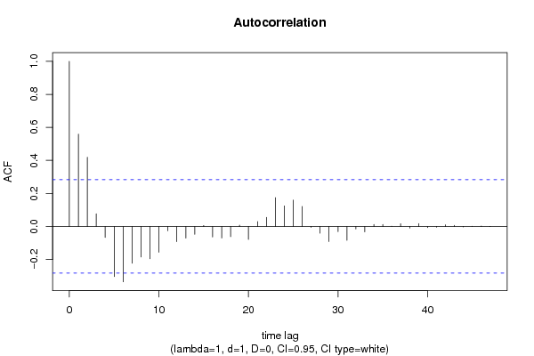
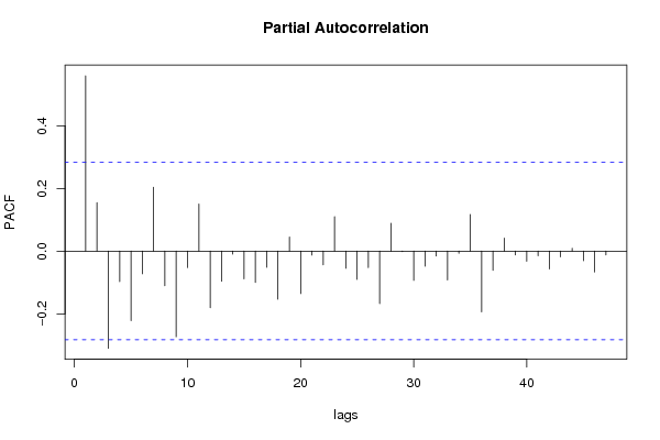
Title produced by software

(Partial) Autocorrelation Function

Date of computation

Tue, 21 Dec 2010 16:00:40 +0000

Cite this page as follows

Statistical Computations at FreeStatistics.org, Office for Research Development and Education, URL https://freestatistics.org/blog/index.php?v=date/2010/Dec/21/t12929471101eoug79li916asu.htm/, Retrieved Sun, 19 May 2024 03:20:03 +0000

Statistical Computations at FreeStatistics.org, Office for Research Development and Education, URL https://freestatistics.org/blog/index.php?pk=113705, Retrieved Sun, 19 May 2024 03:20:03 +0000

QR Codes:

Paste this QR Code to cite your computation.

Original text written by user:

IsPrivate?

No (this computation is public)

User-defined keywords

Estimated Impact

127

Family? (F = Feedback message, R = changed R code, M = changed R Module, P = changed Parameters, D = changed Data)

-     [Univariate Explorative Data Analysis] [Run Sequence gebo...] [2008-12-12 13:32:37] [76963dc1903f0f612b6153510a3818cf]
- R  D  [Univariate Explorative Data Analysis] [Run Sequence gebo...] [2008-12-17 12:14:40] [76963dc1903f0f612b6153510a3818cf]
-         [Univariate Explorative Data Analysis] [Run Sequence Plot...] [2008-12-22 18:19:51] [1ce0d16c8f4225c977b42c8fa93bc163]
- RMP       [Univariate Data Series] [Identifying Integ...] [2009-11-22 12:08:06] [b98453cac15ba1066b407e146608df68]
- RMP         [(Partial) Autocorrelation Function] [Births] [2010-11-29 09:36:27] [b98453cac15ba1066b407e146608df68]
-   PD          [(Partial) Autocorrelation Function] [] [2010-12-20 09:44:34] [94f4aa1c01e87d8321fffb341ed4df07]
-   PD              [(Partial) Autocorrelation Function] [] [2010-12-21 16:00:40] [d1991ab4912b5ede0ff54c26afa5d84c] [Current]

Feedback Forum

Post a new message

Dataseries X:

Download CSV

Histogram

Boxplots

Summary of computational transaction
Raw Input	view raw input (R code)
Raw Output	view raw output of R engine
Computing time	2 seconds
R Server	'Sir Ronald Aylmer Fisher' @ 193.190.124.24

\begin{tabular}{lllllllll}
\hline
Summary of computational transaction \tabularnewline
Raw Input & view raw input (R code)  \tabularnewline
Raw Output & view raw output of R engine  \tabularnewline
Computing time & 2 seconds \tabularnewline
R Server & 'Sir Ronald Aylmer Fisher' @ 193.190.124.24 \tabularnewline
\hline
\end{tabular}
%Source: https://freestatistics.org/blog/index.php?pk=113705&T=0

[TABLE]
[ROW][C]Summary of computational transaction[/C][/ROW]
[ROW][C]Raw Input[/C][C]view raw input (R code) [/C][/ROW]
[ROW][C]Raw Output[/C][C]view raw output of R engine [/C][/ROW]
[ROW][C]Computing time[/C][C]2 seconds[/C][/ROW]
[ROW][C]R Server[/C][C]'Sir Ronald Aylmer Fisher' @ 193.190.124.24[/C][/ROW]
[/TABLE]
Source: https://freestatistics.org/blog/index.php?pk=113705&T=0

Globally Unique Identifier (entire table): ba.freestatistics.org/blog/index.php?pk=113705&T=0

As an alternative you can also use a QR Code:

The GUIDs for individual cells are displayed in the table below:

Summary of computational transaction
Raw Input	view raw input (R code)
Raw Output	view raw output of R engine
Computing time	2 seconds
R Server	'Sir Ronald Aylmer Fisher' @ 193.190.124.24

Autocorrelation Function
Time lag k	ACF(k)	T-STAT	P-value
1	0.559267	3.8747	0.000162
2	0.418993	2.9029	0.002785
3	0.076478	0.5299	0.299328
4	-0.066637	-0.4617	0.323201
5	-0.303871	-2.1053	0.020263
6	-0.335604	-2.3251	0.01217
7	-0.222988	-1.5449	0.064469
8	-0.185052	-1.2821	0.102986
9	-0.196198	-1.3593	0.090202
10	-0.156375	-1.0834	0.142022
11	-0.026396	-0.1829	0.427833
12	-0.092226	-0.639	0.262943
13	-0.070913	-0.4913	0.312728
14	-0.048027	-0.3327	0.370389
15	0.005787	0.0401	0.484092
16	-0.064011	-0.4435	0.329704
17	-0.070198	-0.4863	0.314469
18	-0.061912	-0.4289	0.334943
19	0.008059	0.0558	0.477854
20	-0.078643	-0.5449	0.294189
21	0.028821	0.1997	0.421287
22	0.05543	0.384	0.351325
23	0.174164	1.2066	0.116742
24	0.124288	0.8611	0.196734
25	0.159304	1.1037	0.137615
26	0.121155	0.8394	0.202706
27	-0.005706	-0.0395	0.484315
28	-0.040946	-0.2837	0.388936
29	-0.091689	-0.6352	0.264144
30	-0.032073	-0.2222	0.412548
31	-0.083831	-0.5808	0.282047
32	-0.015458	-0.1071	0.457579
33	-0.033135	-0.2296	0.409702
34	0.01232	0.0854	0.466166
35	0.011496	0.0796	0.468425
36	0.001244	0.0086	0.49658
37	0.016541	0.1146	0.454621
38	-0.010214	-0.0708	0.471939
39	0.01684	0.1167	0.453803
40	-0.006969	-0.0483	0.480846
41	-0.004328	-0.03	0.488102
42	0.009885	0.0685	0.472841
43	0.006573	0.0455	0.481934
44	-0.003626	-0.0251	0.490031
45	-0.000655	-0.0045	0.4982
46	0.002227	0.0154	0.493878
47	-0.001193	-0.0083	0.496719
48	NA	NA	NA

\begin{tabular}{lllllllll}
\hline
Autocorrelation Function \tabularnewline
Time lag k & ACF(k) & T-STAT & P-value \tabularnewline
1 & 0.559267 & 3.8747 & 0.000162 \tabularnewline
2 & 0.418993 & 2.9029 & 0.002785 \tabularnewline
3 & 0.076478 & 0.5299 & 0.299328 \tabularnewline
4 & -0.066637 & -0.4617 & 0.323201 \tabularnewline
5 & -0.303871 & -2.1053 & 0.020263 \tabularnewline
6 & -0.335604 & -2.3251 & 0.01217 \tabularnewline
7 & -0.222988 & -1.5449 & 0.064469 \tabularnewline
8 & -0.185052 & -1.2821 & 0.102986 \tabularnewline
9 & -0.196198 & -1.3593 & 0.090202 \tabularnewline
10 & -0.156375 & -1.0834 & 0.142022 \tabularnewline
11 & -0.026396 & -0.1829 & 0.427833 \tabularnewline
12 & -0.092226 & -0.639 & 0.262943 \tabularnewline
13 & -0.070913 & -0.4913 & 0.312728 \tabularnewline
14 & -0.048027 & -0.3327 & 0.370389 \tabularnewline
15 & 0.005787 & 0.0401 & 0.484092 \tabularnewline
16 & -0.064011 & -0.4435 & 0.329704 \tabularnewline
17 & -0.070198 & -0.4863 & 0.314469 \tabularnewline
18 & -0.061912 & -0.4289 & 0.334943 \tabularnewline
19 & 0.008059 & 0.0558 & 0.477854 \tabularnewline
20 & -0.078643 & -0.5449 & 0.294189 \tabularnewline
21 & 0.028821 & 0.1997 & 0.421287 \tabularnewline
22 & 0.05543 & 0.384 & 0.351325 \tabularnewline
23 & 0.174164 & 1.2066 & 0.116742 \tabularnewline
24 & 0.124288 & 0.8611 & 0.196734 \tabularnewline
25 & 0.159304 & 1.1037 & 0.137615 \tabularnewline
26 & 0.121155 & 0.8394 & 0.202706 \tabularnewline
27 & -0.005706 & -0.0395 & 0.484315 \tabularnewline
28 & -0.040946 & -0.2837 & 0.388936 \tabularnewline
29 & -0.091689 & -0.6352 & 0.264144 \tabularnewline
30 & -0.032073 & -0.2222 & 0.412548 \tabularnewline
31 & -0.083831 & -0.5808 & 0.282047 \tabularnewline
32 & -0.015458 & -0.1071 & 0.457579 \tabularnewline
33 & -0.033135 & -0.2296 & 0.409702 \tabularnewline
34 & 0.01232 & 0.0854 & 0.466166 \tabularnewline
35 & 0.011496 & 0.0796 & 0.468425 \tabularnewline
36 & 0.001244 & 0.0086 & 0.49658 \tabularnewline
37 & 0.016541 & 0.1146 & 0.454621 \tabularnewline
38 & -0.010214 & -0.0708 & 0.471939 \tabularnewline
39 & 0.01684 & 0.1167 & 0.453803 \tabularnewline
40 & -0.006969 & -0.0483 & 0.480846 \tabularnewline
41 & -0.004328 & -0.03 & 0.488102 \tabularnewline
42 & 0.009885 & 0.0685 & 0.472841 \tabularnewline
43 & 0.006573 & 0.0455 & 0.481934 \tabularnewline
44 & -0.003626 & -0.0251 & 0.490031 \tabularnewline
45 & -0.000655 & -0.0045 & 0.4982 \tabularnewline
46 & 0.002227 & 0.0154 & 0.493878 \tabularnewline
47 & -0.001193 & -0.0083 & 0.496719 \tabularnewline
48 & NA & NA & NA \tabularnewline
\hline
\end{tabular}
%Source: https://freestatistics.org/blog/index.php?pk=113705&T=1

[TABLE]
[ROW][C]Autocorrelation Function[/C][/ROW]
[ROW][C]Time lag k[/C][C]ACF(k)[/C][C]T-STAT[/C][C]P-value[/C][/ROW]
[ROW][C]1[/C][C]0.559267[/C][C]3.8747[/C][C]0.000162[/C][/ROW]
[ROW][C]2[/C][C]0.418993[/C][C]2.9029[/C][C]0.002785[/C][/ROW]
[ROW][C]3[/C][C]0.076478[/C][C]0.5299[/C][C]0.299328[/C][/ROW]
[ROW][C]4[/C][C]-0.066637[/C][C]-0.4617[/C][C]0.323201[/C][/ROW]
[ROW][C]5[/C][C]-0.303871[/C][C]-2.1053[/C][C]0.020263[/C][/ROW]
[ROW][C]6[/C][C]-0.335604[/C][C]-2.3251[/C][C]0.01217[/C][/ROW]
[ROW][C]7[/C][C]-0.222988[/C][C]-1.5449[/C][C]0.064469[/C][/ROW]
[ROW][C]8[/C][C]-0.185052[/C][C]-1.2821[/C][C]0.102986[/C][/ROW]
[ROW][C]9[/C][C]-0.196198[/C][C]-1.3593[/C][C]0.090202[/C][/ROW]
[ROW][C]10[/C][C]-0.156375[/C][C]-1.0834[/C][C]0.142022[/C][/ROW]
[ROW][C]11[/C][C]-0.026396[/C][C]-0.1829[/C][C]0.427833[/C][/ROW]
[ROW][C]12[/C][C]-0.092226[/C][C]-0.639[/C][C]0.262943[/C][/ROW]
[ROW][C]13[/C][C]-0.070913[/C][C]-0.4913[/C][C]0.312728[/C][/ROW]
[ROW][C]14[/C][C]-0.048027[/C][C]-0.3327[/C][C]0.370389[/C][/ROW]
[ROW][C]15[/C][C]0.005787[/C][C]0.0401[/C][C]0.484092[/C][/ROW]
[ROW][C]16[/C][C]-0.064011[/C][C]-0.4435[/C][C]0.329704[/C][/ROW]
[ROW][C]17[/C][C]-0.070198[/C][C]-0.4863[/C][C]0.314469[/C][/ROW]
[ROW][C]18[/C][C]-0.061912[/C][C]-0.4289[/C][C]0.334943[/C][/ROW]
[ROW][C]19[/C][C]0.008059[/C][C]0.0558[/C][C]0.477854[/C][/ROW]
[ROW][C]20[/C][C]-0.078643[/C][C]-0.5449[/C][C]0.294189[/C][/ROW]
[ROW][C]21[/C][C]0.028821[/C][C]0.1997[/C][C]0.421287[/C][/ROW]
[ROW][C]22[/C][C]0.05543[/C][C]0.384[/C][C]0.351325[/C][/ROW]
[ROW][C]23[/C][C]0.174164[/C][C]1.2066[/C][C]0.116742[/C][/ROW]
[ROW][C]24[/C][C]0.124288[/C][C]0.8611[/C][C]0.196734[/C][/ROW]
[ROW][C]25[/C][C]0.159304[/C][C]1.1037[/C][C]0.137615[/C][/ROW]
[ROW][C]26[/C][C]0.121155[/C][C]0.8394[/C][C]0.202706[/C][/ROW]
[ROW][C]27[/C][C]-0.005706[/C][C]-0.0395[/C][C]0.484315[/C][/ROW]
[ROW][C]28[/C][C]-0.040946[/C][C]-0.2837[/C][C]0.388936[/C][/ROW]
[ROW][C]29[/C][C]-0.091689[/C][C]-0.6352[/C][C]0.264144[/C][/ROW]
[ROW][C]30[/C][C]-0.032073[/C][C]-0.2222[/C][C]0.412548[/C][/ROW]
[ROW][C]31[/C][C]-0.083831[/C][C]-0.5808[/C][C]0.282047[/C][/ROW]
[ROW][C]32[/C][C]-0.015458[/C][C]-0.1071[/C][C]0.457579[/C][/ROW]
[ROW][C]33[/C][C]-0.033135[/C][C]-0.2296[/C][C]0.409702[/C][/ROW]
[ROW][C]34[/C][C]0.01232[/C][C]0.0854[/C][C]0.466166[/C][/ROW]
[ROW][C]35[/C][C]0.011496[/C][C]0.0796[/C][C]0.468425[/C][/ROW]
[ROW][C]36[/C][C]0.001244[/C][C]0.0086[/C][C]0.49658[/C][/ROW]
[ROW][C]37[/C][C]0.016541[/C][C]0.1146[/C][C]0.454621[/C][/ROW]
[ROW][C]38[/C][C]-0.010214[/C][C]-0.0708[/C][C]0.471939[/C][/ROW]
[ROW][C]39[/C][C]0.01684[/C][C]0.1167[/C][C]0.453803[/C][/ROW]
[ROW][C]40[/C][C]-0.006969[/C][C]-0.0483[/C][C]0.480846[/C][/ROW]
[ROW][C]41[/C][C]-0.004328[/C][C]-0.03[/C][C]0.488102[/C][/ROW]
[ROW][C]42[/C][C]0.009885[/C][C]0.0685[/C][C]0.472841[/C][/ROW]
[ROW][C]43[/C][C]0.006573[/C][C]0.0455[/C][C]0.481934[/C][/ROW]
[ROW][C]44[/C][C]-0.003626[/C][C]-0.0251[/C][C]0.490031[/C][/ROW]
[ROW][C]45[/C][C]-0.000655[/C][C]-0.0045[/C][C]0.4982[/C][/ROW]
[ROW][C]46[/C][C]0.002227[/C][C]0.0154[/C][C]0.493878[/C][/ROW]
[ROW][C]47[/C][C]-0.001193[/C][C]-0.0083[/C][C]0.496719[/C][/ROW]
[ROW][C]48[/C][C]NA[/C][C]NA[/C][C]NA[/C][/ROW]
[/TABLE]
Source: https://freestatistics.org/blog/index.php?pk=113705&T=1

Globally Unique Identifier (entire table): ba.freestatistics.org/blog/index.php?pk=113705&T=1

As an alternative you can also use a QR Code:

The GUIDs for individual cells are displayed in the table below:

Autocorrelation Function
Time lag k	ACF(k)	T-STAT	P-value
1	0.559267	3.8747	0.000162
2	0.418993	2.9029	0.002785
3	0.076478	0.5299	0.299328
4	-0.066637	-0.4617	0.323201
5	-0.303871	-2.1053	0.020263
6	-0.335604	-2.3251	0.01217
7	-0.222988	-1.5449	0.064469
8	-0.185052	-1.2821	0.102986
9	-0.196198	-1.3593	0.090202
10	-0.156375	-1.0834	0.142022
11	-0.026396	-0.1829	0.427833
12	-0.092226	-0.639	0.262943
13	-0.070913	-0.4913	0.312728
14	-0.048027	-0.3327	0.370389
15	0.005787	0.0401	0.484092
16	-0.064011	-0.4435	0.329704
17	-0.070198	-0.4863	0.314469
18	-0.061912	-0.4289	0.334943
19	0.008059	0.0558	0.477854
20	-0.078643	-0.5449	0.294189
21	0.028821	0.1997	0.421287
22	0.05543	0.384	0.351325
23	0.174164	1.2066	0.116742
24	0.124288	0.8611	0.196734
25	0.159304	1.1037	0.137615
26	0.121155	0.8394	0.202706
27	-0.005706	-0.0395	0.484315
28	-0.040946	-0.2837	0.388936
29	-0.091689	-0.6352	0.264144
30	-0.032073	-0.2222	0.412548
31	-0.083831	-0.5808	0.282047
32	-0.015458	-0.1071	0.457579
33	-0.033135	-0.2296	0.409702
34	0.01232	0.0854	0.466166
35	0.011496	0.0796	0.468425
36	0.001244	0.0086	0.49658
37	0.016541	0.1146	0.454621
38	-0.010214	-0.0708	0.471939
39	0.01684	0.1167	0.453803
40	-0.006969	-0.0483	0.480846
41	-0.004328	-0.03	0.488102
42	0.009885	0.0685	0.472841
43	0.006573	0.0455	0.481934
44	-0.003626	-0.0251	0.490031
45	-0.000655	-0.0045	0.4982
46	0.002227	0.0154	0.493878
47	-0.001193	-0.0083	0.496719
48	NA	NA	NA

Partial Autocorrelation Function
Time lag k	PACF(k)	T-STAT	P-value
1	0.559267	3.8747	0.000162
2	0.154556	1.0708	0.144809
3	-0.310183	-2.149	0.018353
4	-0.097643	-0.6765	0.250988
5	-0.22183	-1.5369	0.065444
6	-0.072396	-0.5016	0.30913
7	0.203807	1.412	0.082197
8	-0.110455	-0.7653	0.223934
9	-0.273277	-1.8933	0.032176
10	-0.05297	-0.367	0.357621
11	0.150259	1.041	0.15154
12	-0.180549	-1.2509	0.108521
13	-0.096078	-0.6656	0.254412
14	-0.009631	-0.0667	0.473538
15	-0.088893	-0.6159	0.270445
16	-0.100123	-0.6937	0.245615
17	-0.051885	-0.3595	0.36041
18	-0.153824	-1.0657	0.14594
19	0.045085	0.3124	0.378061
20	-0.135597	-0.9394	0.176104
21	-0.012811	-0.0888	0.464823
22	-0.044025	-0.305	0.380837
23	0.10965	0.7597	0.225581
24	-0.054841	-0.38	0.352829
25	-0.090701	-0.6284	0.266362
26	-0.052675	-0.3649	0.358378
27	-0.167403	-1.1598	0.125933
28	0.089164	0.6177	0.26983
29	-0.001572	-0.0109	0.495676
30	-0.093547	-0.6481	0.260001
31	-0.048496	-0.336	0.369171
32	-0.01569	-0.1087	0.456945
33	-0.091932	-0.6369	0.263601
34	-0.00705	-0.0488	0.480624
35	0.116714	0.8086	0.211361
36	-0.193704	-1.342	0.092952
37	-0.061277	-0.4245	0.336535
38	0.041398	0.2868	0.387745
39	-0.012406	-0.086	0.46593
40	-0.032203	-0.2231	0.4122
41	-0.015048	-0.1043	0.4587
42	-0.056798	-0.3935	0.347844
43	-0.018516	-0.1283	0.449232
44	0.008845	0.0613	0.475696
45	-0.030471	-0.2111	0.416849
46	-0.06687	-0.4633	0.322627
47	-0.012375	-0.0857	0.466016
48	NA	NA	NA

\begin{tabular}{lllllllll}
\hline
Partial Autocorrelation Function \tabularnewline
Time lag k & PACF(k) & T-STAT & P-value \tabularnewline
1 & 0.559267 & 3.8747 & 0.000162 \tabularnewline
2 & 0.154556 & 1.0708 & 0.144809 \tabularnewline
3 & -0.310183 & -2.149 & 0.018353 \tabularnewline
4 & -0.097643 & -0.6765 & 0.250988 \tabularnewline
5 & -0.22183 & -1.5369 & 0.065444 \tabularnewline
6 & -0.072396 & -0.5016 & 0.30913 \tabularnewline
7 & 0.203807 & 1.412 & 0.082197 \tabularnewline
8 & -0.110455 & -0.7653 & 0.223934 \tabularnewline
9 & -0.273277 & -1.8933 & 0.032176 \tabularnewline
10 & -0.05297 & -0.367 & 0.357621 \tabularnewline
11 & 0.150259 & 1.041 & 0.15154 \tabularnewline
12 & -0.180549 & -1.2509 & 0.108521 \tabularnewline
13 & -0.096078 & -0.6656 & 0.254412 \tabularnewline
14 & -0.009631 & -0.0667 & 0.473538 \tabularnewline
15 & -0.088893 & -0.6159 & 0.270445 \tabularnewline
16 & -0.100123 & -0.6937 & 0.245615 \tabularnewline
17 & -0.051885 & -0.3595 & 0.36041 \tabularnewline
18 & -0.153824 & -1.0657 & 0.14594 \tabularnewline
19 & 0.045085 & 0.3124 & 0.378061 \tabularnewline
20 & -0.135597 & -0.9394 & 0.176104 \tabularnewline
21 & -0.012811 & -0.0888 & 0.464823 \tabularnewline
22 & -0.044025 & -0.305 & 0.380837 \tabularnewline
23 & 0.10965 & 0.7597 & 0.225581 \tabularnewline
24 & -0.054841 & -0.38 & 0.352829 \tabularnewline
25 & -0.090701 & -0.6284 & 0.266362 \tabularnewline
26 & -0.052675 & -0.3649 & 0.358378 \tabularnewline
27 & -0.167403 & -1.1598 & 0.125933 \tabularnewline
28 & 0.089164 & 0.6177 & 0.26983 \tabularnewline
29 & -0.001572 & -0.0109 & 0.495676 \tabularnewline
30 & -0.093547 & -0.6481 & 0.260001 \tabularnewline
31 & -0.048496 & -0.336 & 0.369171 \tabularnewline
32 & -0.01569 & -0.1087 & 0.456945 \tabularnewline
33 & -0.091932 & -0.6369 & 0.263601 \tabularnewline
34 & -0.00705 & -0.0488 & 0.480624 \tabularnewline
35 & 0.116714 & 0.8086 & 0.211361 \tabularnewline
36 & -0.193704 & -1.342 & 0.092952 \tabularnewline
37 & -0.061277 & -0.4245 & 0.336535 \tabularnewline
38 & 0.041398 & 0.2868 & 0.387745 \tabularnewline
39 & -0.012406 & -0.086 & 0.46593 \tabularnewline
40 & -0.032203 & -0.2231 & 0.4122 \tabularnewline
41 & -0.015048 & -0.1043 & 0.4587 \tabularnewline
42 & -0.056798 & -0.3935 & 0.347844 \tabularnewline
43 & -0.018516 & -0.1283 & 0.449232 \tabularnewline
44 & 0.008845 & 0.0613 & 0.475696 \tabularnewline
45 & -0.030471 & -0.2111 & 0.416849 \tabularnewline
46 & -0.06687 & -0.4633 & 0.322627 \tabularnewline
47 & -0.012375 & -0.0857 & 0.466016 \tabularnewline
48 & NA & NA & NA \tabularnewline
\hline
\end{tabular}
%Source: https://freestatistics.org/blog/index.php?pk=113705&T=2

[TABLE]
[ROW][C]Partial Autocorrelation Function[/C][/ROW]
[ROW][C]Time lag k[/C][C]PACF(k)[/C][C]T-STAT[/C][C]P-value[/C][/ROW]
[ROW][C]1[/C][C]0.559267[/C][C]3.8747[/C][C]0.000162[/C][/ROW]
[ROW][C]2[/C][C]0.154556[/C][C]1.0708[/C][C]0.144809[/C][/ROW]
[ROW][C]3[/C][C]-0.310183[/C][C]-2.149[/C][C]0.018353[/C][/ROW]
[ROW][C]4[/C][C]-0.097643[/C][C]-0.6765[/C][C]0.250988[/C][/ROW]
[ROW][C]5[/C][C]-0.22183[/C][C]-1.5369[/C][C]0.065444[/C][/ROW]
[ROW][C]6[/C][C]-0.072396[/C][C]-0.5016[/C][C]0.30913[/C][/ROW]
[ROW][C]7[/C][C]0.203807[/C][C]1.412[/C][C]0.082197[/C][/ROW]
[ROW][C]8[/C][C]-0.110455[/C][C]-0.7653[/C][C]0.223934[/C][/ROW]
[ROW][C]9[/C][C]-0.273277[/C][C]-1.8933[/C][C]0.032176[/C][/ROW]
[ROW][C]10[/C][C]-0.05297[/C][C]-0.367[/C][C]0.357621[/C][/ROW]
[ROW][C]11[/C][C]0.150259[/C][C]1.041[/C][C]0.15154[/C][/ROW]
[ROW][C]12[/C][C]-0.180549[/C][C]-1.2509[/C][C]0.108521[/C][/ROW]
[ROW][C]13[/C][C]-0.096078[/C][C]-0.6656[/C][C]0.254412[/C][/ROW]
[ROW][C]14[/C][C]-0.009631[/C][C]-0.0667[/C][C]0.473538[/C][/ROW]
[ROW][C]15[/C][C]-0.088893[/C][C]-0.6159[/C][C]0.270445[/C][/ROW]
[ROW][C]16[/C][C]-0.100123[/C][C]-0.6937[/C][C]0.245615[/C][/ROW]
[ROW][C]17[/C][C]-0.051885[/C][C]-0.3595[/C][C]0.36041[/C][/ROW]
[ROW][C]18[/C][C]-0.153824[/C][C]-1.0657[/C][C]0.14594[/C][/ROW]
[ROW][C]19[/C][C]0.045085[/C][C]0.3124[/C][C]0.378061[/C][/ROW]
[ROW][C]20[/C][C]-0.135597[/C][C]-0.9394[/C][C]0.176104[/C][/ROW]
[ROW][C]21[/C][C]-0.012811[/C][C]-0.0888[/C][C]0.464823[/C][/ROW]
[ROW][C]22[/C][C]-0.044025[/C][C]-0.305[/C][C]0.380837[/C][/ROW]
[ROW][C]23[/C][C]0.10965[/C][C]0.7597[/C][C]0.225581[/C][/ROW]
[ROW][C]24[/C][C]-0.054841[/C][C]-0.38[/C][C]0.352829[/C][/ROW]
[ROW][C]25[/C][C]-0.090701[/C][C]-0.6284[/C][C]0.266362[/C][/ROW]
[ROW][C]26[/C][C]-0.052675[/C][C]-0.3649[/C][C]0.358378[/C][/ROW]
[ROW][C]27[/C][C]-0.167403[/C][C]-1.1598[/C][C]0.125933[/C][/ROW]
[ROW][C]28[/C][C]0.089164[/C][C]0.6177[/C][C]0.26983[/C][/ROW]
[ROW][C]29[/C][C]-0.001572[/C][C]-0.0109[/C][C]0.495676[/C][/ROW]
[ROW][C]30[/C][C]-0.093547[/C][C]-0.6481[/C][C]0.260001[/C][/ROW]
[ROW][C]31[/C][C]-0.048496[/C][C]-0.336[/C][C]0.369171[/C][/ROW]
[ROW][C]32[/C][C]-0.01569[/C][C]-0.1087[/C][C]0.456945[/C][/ROW]
[ROW][C]33[/C][C]-0.091932[/C][C]-0.6369[/C][C]0.263601[/C][/ROW]
[ROW][C]34[/C][C]-0.00705[/C][C]-0.0488[/C][C]0.480624[/C][/ROW]
[ROW][C]35[/C][C]0.116714[/C][C]0.8086[/C][C]0.211361[/C][/ROW]
[ROW][C]36[/C][C]-0.193704[/C][C]-1.342[/C][C]0.092952[/C][/ROW]
[ROW][C]37[/C][C]-0.061277[/C][C]-0.4245[/C][C]0.336535[/C][/ROW]
[ROW][C]38[/C][C]0.041398[/C][C]0.2868[/C][C]0.387745[/C][/ROW]
[ROW][C]39[/C][C]-0.012406[/C][C]-0.086[/C][C]0.46593[/C][/ROW]
[ROW][C]40[/C][C]-0.032203[/C][C]-0.2231[/C][C]0.4122[/C][/ROW]
[ROW][C]41[/C][C]-0.015048[/C][C]-0.1043[/C][C]0.4587[/C][/ROW]
[ROW][C]42[/C][C]-0.056798[/C][C]-0.3935[/C][C]0.347844[/C][/ROW]
[ROW][C]43[/C][C]-0.018516[/C][C]-0.1283[/C][C]0.449232[/C][/ROW]
[ROW][C]44[/C][C]0.008845[/C][C]0.0613[/C][C]0.475696[/C][/ROW]
[ROW][C]45[/C][C]-0.030471[/C][C]-0.2111[/C][C]0.416849[/C][/ROW]
[ROW][C]46[/C][C]-0.06687[/C][C]-0.4633[/C][C]0.322627[/C][/ROW]
[ROW][C]47[/C][C]-0.012375[/C][C]-0.0857[/C][C]0.466016[/C][/ROW]
[ROW][C]48[/C][C]NA[/C][C]NA[/C][C]NA[/C][/ROW]
[/TABLE]
Source: https://freestatistics.org/blog/index.php?pk=113705&T=2

Globally Unique Identifier (entire table): ba.freestatistics.org/blog/index.php?pk=113705&T=2

As an alternative you can also use a QR Code:

The GUIDs for individual cells are displayed in the table below:

Partial Autocorrelation Function
Time lag k	PACF(k)	T-STAT	P-value
1	0.559267	3.8747	0.000162
2	0.154556	1.0708	0.144809
3	-0.310183	-2.149	0.018353
4	-0.097643	-0.6765	0.250988
5	-0.22183	-1.5369	0.065444
6	-0.072396	-0.5016	0.30913
7	0.203807	1.412	0.082197
8	-0.110455	-0.7653	0.223934
9	-0.273277	-1.8933	0.032176
10	-0.05297	-0.367	0.357621
11	0.150259	1.041	0.15154
12	-0.180549	-1.2509	0.108521
13	-0.096078	-0.6656	0.254412
14	-0.009631	-0.0667	0.473538
15	-0.088893	-0.6159	0.270445
16	-0.100123	-0.6937	0.245615
17	-0.051885	-0.3595	0.36041
18	-0.153824	-1.0657	0.14594
19	0.045085	0.3124	0.378061
20	-0.135597	-0.9394	0.176104
21	-0.012811	-0.0888	0.464823
22	-0.044025	-0.305	0.380837
23	0.10965	0.7597	0.225581
24	-0.054841	-0.38	0.352829
25	-0.090701	-0.6284	0.266362
26	-0.052675	-0.3649	0.358378
27	-0.167403	-1.1598	0.125933
28	0.089164	0.6177	0.26983
29	-0.001572	-0.0109	0.495676
30	-0.093547	-0.6481	0.260001
31	-0.048496	-0.336	0.369171
32	-0.01569	-0.1087	0.456945
33	-0.091932	-0.6369	0.263601
34	-0.00705	-0.0488	0.480624
35	0.116714	0.8086	0.211361
36	-0.193704	-1.342	0.092952
37	-0.061277	-0.4245	0.336535
38	0.041398	0.2868	0.387745
39	-0.012406	-0.086	0.46593
40	-0.032203	-0.2231	0.4122
41	-0.015048	-0.1043	0.4587
42	-0.056798	-0.3935	0.347844
43	-0.018516	-0.1283	0.449232
44	0.008845	0.0613	0.475696
45	-0.030471	-0.2111	0.416849
46	-0.06687	-0.4633	0.322627
47	-0.012375	-0.0857	0.466016
48	NA	NA	NA

Figure 1

PNG link

Postscript link

PDF link

Figure 2

PNG link

Postscript link

PDF link

Parameters (Session):

par1 = 48 ; par2 = 1 ; par3 = 1 ; par4 = 0 ; par5 = 12 ; par6 = White Noise ; par7 = 0.95 ;

Parameters (R input):

par1 = 48 ; par2 = 1 ; par3 = 1 ; par4 = 0 ; par5 = 12 ; par6 = White Noise ; par7 = 0.95 ; par8 = ;

R code (references can be found in the software module):

if (par1 == 'Default') {
par1 = 10*log10(length(x))
} else {
par1 <- as.numeric(par1)
}
par2 <- as.numeric(par2)
par3 <- as.numeric(par3)
par4 <- as.numeric(par4)
par5 <- as.numeric(par5)
if (par6 == 'White Noise') par6 <- 'white' else par6 <- 'ma'
par7 <- as.numeric(par7)
if (par2 == 0) {
x <- log(x)
} else {
x <- (x ^ par2 - 1) / par2
}
if (par3 > 0) x <- diff(x,lag=1,difference=par3)
if (par4 > 0) x <- diff(x,lag=par5,difference=par4)
bitmap(file='pic1.png')
racf <- acf(x, par1, main='Autocorrelation', xlab='time lag', ylab='ACF', ci.type=par6, ci=par7, sub=paste('(lambda=',par2,', d=',par3,', D=',par4,', CI=', par7, ', CI type=',par6,')',sep=''))
dev.off()
bitmap(file='pic2.png')
rpacf <- pacf(x,par1,main='Partial Autocorrelation',xlab='lags',ylab='PACF')
dev.off()
(myacf <- c(racf$acf))
(mypacf <- c(rpacf$acf))
lengthx <- length(x)
sqrtn <- sqrt(lengthx)
load(file='createtable')
a<-table.start()
a<-table.row.start(a)
a<-table.element(a,'Autocorrelation Function',4,TRUE)
a<-table.row.end(a)
a<-table.row.start(a)
a<-table.element(a,'Time lag k',header=TRUE)
a<-table.element(a,hyperlink('basics.htm','ACF(k)','click here for more information about the Autocorrelation Function'),header=TRUE)
a<-table.element(a,'T-STAT',header=TRUE)
a<-table.element(a,'P-value',header=TRUE)
a<-table.row.end(a)
for (i in 2:(par1+1)) {
a<-table.row.start(a)
a<-table.element(a,i-1,header=TRUE)
a<-table.element(a,round(myacf[i],6))
mytstat <- myacf[i]*sqrtn
a<-table.element(a,round(mytstat,4))
a<-table.element(a,round(1-pt(abs(mytstat),lengthx),6))
a<-table.row.end(a)
}
a<-table.end(a)
table.save(a,file='mytable.tab')
a<-table.start()
a<-table.row.start(a)
a<-table.element(a,'Partial Autocorrelation Function',4,TRUE)
a<-table.row.end(a)
a<-table.row.start(a)
a<-table.element(a,'Time lag k',header=TRUE)
a<-table.element(a,hyperlink('basics.htm','PACF(k)','click here for more information about the Partial Autocorrelation Function'),header=TRUE)
a<-table.element(a,'T-STAT',header=TRUE)
a<-table.element(a,'P-value',header=TRUE)
a<-table.row.end(a)
for (i in 1:par1) {
a<-table.row.start(a)
a<-table.element(a,i,header=TRUE)
a<-table.element(a,round(mypacf[i],6))
mytstat <- mypacf[i]*sqrtn
a<-table.element(a,round(mytstat,4))
a<-table.element(a,round(1-pt(abs(mytstat),lengthx),6))
a<-table.row.end(a)
}
a<-table.end(a)
table.save(a,file='mytable1.tab')

Free Statistics

Description of Statistical Computation

Tree of Dependent Computations

Dataset

Tables (Output of Computation)

Figures (Output of Computation)

Input Parameters & R Code