Free Statistics

of Irreproducible Research!

Author's title

Author*The author of this computation has been verified*
R Software Modulerwasp_percentiles.wasp
Title produced by softwarePercentiles
Date of computationMon, 20 Oct 2008 12:53:19 -0600
Cite this page as followsStatistical Computations at FreeStatistics.org, Office for Research Development and Education, URL https://freestatistics.org/blog/index.php?v=date/2008/Oct/20/t12245288588q5o7oy5po11id3.htm/, Retrieved Fri, 17 May 2024 07:56:51 +0000
Statistical Computations at FreeStatistics.org, Office for Research Development and Education, URL https://freestatistics.org/blog/index.php?pk=17897, Retrieved Fri, 17 May 2024 07:56:51 +0000
QR Codes:

Original text written by user:
IsPrivate?No (this computation is public)
User-defined keywords
Estimated Impact157
Family? (F = Feedback message, R = changed R code, M = changed R Module, P = changed Parameters, D = changed Data)
F     [Percentiles and Normal Probability Plot] [Q6 P(a
F RM D    [Percentiles] [Q6 Percentiles] [2008-10-20 18:53:19] [d7f41258beeebb8716e3f5d39f3cdc01] [Current]
Feedback Forum
2008-10-24 13:06:25 [66991d38d6a4b2d9fe97b6c889f3689c] [reply
De waarde van a kan men aflezen naast 0,10 in de eerste kolom in de link. De waarde voor b kan men aflezen naast 0,90 eveneens in de eerste kolom in de link. Er wordt gevraagd naar een 80% kans dat de waarde tussen a en b ligt. Daarom moet men ook telkens 10 % wegdoen bovenaan en onderaan (100 – 80 = 20/2 = 10). de getallen die men vindt naast 0.10 en 0.90 bepalen het interval.
alle waarden die voorkomen voorbij de waarde bij het 0.10 percentiel, hebben 90% kans om voor te komen. hetzelfde geld voor het 0.90 pencentiel voor de waarden erboven. door langs beide uitersten 10% af te nemen beperkt men de kans tot 80%.
2008-10-26 10:58:47 [339a57d8a4d5d113e4804fc423e4a59e] [reply
De student heeft de percentielen uitgerekent van de gebruikte reeks. Hij is echter niet tot een oplossing van de vraag gekomen. Om deze vraag correct op te lossen moest hij langs weerskanten een deel van 10% 'afkappen', zo bekwam hij een 80% interval. Men moest de twee waarden(a&b) berekenen om deze 80% te bekomen. De eerste waarde (a) bevond zich in de tabel naast het percentiel 0,10(10% afgekapt langs boven). De tweede waarde (b) bevond zich in de tabel naast het percentiel 0,90(10% afgekapt langs onder). De waarden a en b zijn dus respectievelijk 89.98 en 111.67

Post a new message
Dataseries X:
110.40
96.40
101.90
106.20
81.00
94.70
101.00
109.40
102.30
90.70
96.20
96.10
106.00
103.10
102.00
104.70
86.00
92.10
106.90
112.60
101.70
92.00
97.40
97.00
105.40
102.70
98.10
104.50
87.40
89.90
109.80
111.70
98.60
96.90
95.10
97.00
112.70
102.90
97.40
111.40
87.40
96.80
114.10
110.30
103.90
101.60
94.60
95.90
104.70
102.80
98.10
113.90
80.90
95.70
113.20
105.90
108.80
102.30
99.00
100.70
115.50


Summary of computational transaction
Raw Inputview raw input (R code)
Raw Outputview raw output of R engine
Computing time1 seconds
R Server'George Udny Yule' @ 72.249.76.132

\begin{tabular}{lllllllll}
\hline
Summary of computational transaction \tabularnewline
Raw Input & view raw input (R code)  \tabularnewline
Raw Output & view raw output of R engine  \tabularnewline
Computing time & 1 seconds \tabularnewline
R Server & 'George Udny Yule' @ 72.249.76.132 \tabularnewline
\hline
\end{tabular}
%Source: https://freestatistics.org/blog/index.php?pk=17897&T=0

[TABLE]
[ROW][C]Summary of computational transaction[/C][/ROW]
[ROW][C]Raw Input[/C][C]view raw input (R code) [/C][/ROW]
[ROW][C]Raw Output[/C][C]view raw output of R engine [/C][/ROW]
[ROW][C]Computing time[/C][C]1 seconds[/C][/ROW]
[ROW][C]R Server[/C][C]'George Udny Yule' @ 72.249.76.132[/C][/ROW]
[/TABLE]
Source: https://freestatistics.org/blog/index.php?pk=17897&T=0

Globally Unique Identifier (entire table): ba.freestatistics.org/blog/index.php?pk=17897&T=0

As an alternative you can also use a QR Code:  

The GUIDs for individual cells are displayed in the table below:

Summary of computational transaction
Raw Inputview raw input (R code)
Raw Outputview raw output of R engine
Computing time1 seconds
R Server'George Udny Yule' @ 72.249.76.132


Percentiles - Ungrouped Data
pWeighted Average at XnpWeighted Average at X(n+1)pEmpirical Distribution FunctionEmpirical Distribution Function - AveragingEmpirical Distribution Function - InterpolationClosest ObservationTrue Basic - Statistics Graphics ToolkitMS Excel (old versions)
0.0280.92280.92481818280.980.97680.9
0.0483.283.4868686.568183.681
0.0686.92487.00887.487.487.487.486.39287.4
0.0887.487.487.487.489.487.487.487.4
0.189.9890.0690.790.790.789.990.5489.9
0.1291.11691.272929292.0290.791.42890.7
0.1492.05492.06892.192.193.192.192.03292.1
0.169494.494.694.694.6694.692.394.6
0.1894.69894.76494.794.795.0294.795.03694.7
0.295.2295.3495.795.795.795.195.4695.1
0.2295.78495.82895.995.995.9495.795.77295.9
0.2496.02896.07696.196.196.1496.195.92496.1
0.2696.18696.22496.296.296.3296.296.37696.2
0.2896.43296.54496.896.896.7296.496.65696.4
0.396.8396.8696.996.996.996.896.8496.9
0.3296.95296.9849797979796.91697
0.349797.032979797.169797.36897
0.3697.38497.497.497.497.497.497.497.4
0.3897.52697.79298.198.197.9697.497.70898.1
0.498.198.198.198.198.198.198.198.1
0.4298.4198.61698.698.698.6898.698.98498.6
0.4498.93699.476999999.6899100.22499
0.46100.718100.856101101100.88100.7100.844101
0.48101.168101.456101.6101.6101.48101101.144101.6
0.5101.65101.7101.7101.7101.7101.7101.7101.7
0.52101.844101.924101.9101.9101.92101.9101.976101.9
0.54101.994102.144102102102.12102102.156102
0.56102.3102.3102.3102.3102.3102.3102.3102.3
0.58102.452102.684102.7102.7102.62102.3102.316102.7
0.6102.76102.82102.8102.8102.8102.8102.88102.8
0.62102.882102.988102.9102.9102.94102.9103.012102.9
0.64103.132103.644103.9103.9103.42103.1103.356103.9
0.66104.056104.452104.5104.5104.26103.9103.948104.5
0.68104.596104.7104.7104.7104.66104.5104.7104.7
0.7104.7104.98104.7104.7104.7104.7105.12104.7
0.72105.344105.72105.4105.4105.5105.4105.58105.9
0.74105.914105.988106106105.94105.9105.912106
0.76106.072106.284106.2106.2106.12106106.816106.2
0.78106.606107.584106.9106.9106.76106.9108.116106.9
0.8108.42109.16108.8108.8108.8108.8109.04109.4
0.82109.408109.736109.8109.8109.48109.4109.464109.8
0.84109.92110.308110.3110.3110109.8110.392110.3
0.86110.346110.72110.4110.4110.36110.3111.08110.4
0.88111.08111.568111.4111.4111.2111.4111.532111.7
0.9111.67112.42111.7111.7111.7111.7111.88112.6
0.92112.612112.72112.7112.7112.62112.6113.18112.7
0.94112.87113.396113.2113.2112.9112.7113.704113.2
0.96113.592114.004113.9113.9113.62113.9113.996114.1
0.98114.056115.164114.1114.1114.06114.1114.436115.5

\begin{tabular}{lllllllll}
\hline
Percentiles - Ungrouped Data \tabularnewline
p & Weighted Average at Xnp & Weighted Average at X(n+1)p & Empirical Distribution Function & Empirical Distribution Function - Averaging & Empirical Distribution Function - Interpolation & Closest Observation & True Basic - Statistics Graphics Toolkit & MS Excel (old versions) \tabularnewline
0.02 & 80.922 & 80.924 & 81 & 81 & 82 & 80.9 & 80.976 & 80.9 \tabularnewline
0.04 & 83.2 & 83.4 & 86 & 86 & 86.56 & 81 & 83.6 & 81 \tabularnewline
0.06 & 86.924 & 87.008 & 87.4 & 87.4 & 87.4 & 87.4 & 86.392 & 87.4 \tabularnewline
0.08 & 87.4 & 87.4 & 87.4 & 87.4 & 89.4 & 87.4 & 87.4 & 87.4 \tabularnewline
0.1 & 89.98 & 90.06 & 90.7 & 90.7 & 90.7 & 89.9 & 90.54 & 89.9 \tabularnewline
0.12 & 91.116 & 91.272 & 92 & 92 & 92.02 & 90.7 & 91.428 & 90.7 \tabularnewline
0.14 & 92.054 & 92.068 & 92.1 & 92.1 & 93.1 & 92.1 & 92.032 & 92.1 \tabularnewline
0.16 & 94 & 94.4 & 94.6 & 94.6 & 94.66 & 94.6 & 92.3 & 94.6 \tabularnewline
0.18 & 94.698 & 94.764 & 94.7 & 94.7 & 95.02 & 94.7 & 95.036 & 94.7 \tabularnewline
0.2 & 95.22 & 95.34 & 95.7 & 95.7 & 95.7 & 95.1 & 95.46 & 95.1 \tabularnewline
0.22 & 95.784 & 95.828 & 95.9 & 95.9 & 95.94 & 95.7 & 95.772 & 95.9 \tabularnewline
0.24 & 96.028 & 96.076 & 96.1 & 96.1 & 96.14 & 96.1 & 95.924 & 96.1 \tabularnewline
0.26 & 96.186 & 96.224 & 96.2 & 96.2 & 96.32 & 96.2 & 96.376 & 96.2 \tabularnewline
0.28 & 96.432 & 96.544 & 96.8 & 96.8 & 96.72 & 96.4 & 96.656 & 96.4 \tabularnewline
0.3 & 96.83 & 96.86 & 96.9 & 96.9 & 96.9 & 96.8 & 96.84 & 96.9 \tabularnewline
0.32 & 96.952 & 96.984 & 97 & 97 & 97 & 97 & 96.916 & 97 \tabularnewline
0.34 & 97 & 97.032 & 97 & 97 & 97.16 & 97 & 97.368 & 97 \tabularnewline
0.36 & 97.384 & 97.4 & 97.4 & 97.4 & 97.4 & 97.4 & 97.4 & 97.4 \tabularnewline
0.38 & 97.526 & 97.792 & 98.1 & 98.1 & 97.96 & 97.4 & 97.708 & 98.1 \tabularnewline
0.4 & 98.1 & 98.1 & 98.1 & 98.1 & 98.1 & 98.1 & 98.1 & 98.1 \tabularnewline
0.42 & 98.41 & 98.616 & 98.6 & 98.6 & 98.68 & 98.6 & 98.984 & 98.6 \tabularnewline
0.44 & 98.936 & 99.476 & 99 & 99 & 99.68 & 99 & 100.224 & 99 \tabularnewline
0.46 & 100.718 & 100.856 & 101 & 101 & 100.88 & 100.7 & 100.844 & 101 \tabularnewline
0.48 & 101.168 & 101.456 & 101.6 & 101.6 & 101.48 & 101 & 101.144 & 101.6 \tabularnewline
0.5 & 101.65 & 101.7 & 101.7 & 101.7 & 101.7 & 101.7 & 101.7 & 101.7 \tabularnewline
0.52 & 101.844 & 101.924 & 101.9 & 101.9 & 101.92 & 101.9 & 101.976 & 101.9 \tabularnewline
0.54 & 101.994 & 102.144 & 102 & 102 & 102.12 & 102 & 102.156 & 102 \tabularnewline
0.56 & 102.3 & 102.3 & 102.3 & 102.3 & 102.3 & 102.3 & 102.3 & 102.3 \tabularnewline
0.58 & 102.452 & 102.684 & 102.7 & 102.7 & 102.62 & 102.3 & 102.316 & 102.7 \tabularnewline
0.6 & 102.76 & 102.82 & 102.8 & 102.8 & 102.8 & 102.8 & 102.88 & 102.8 \tabularnewline
0.62 & 102.882 & 102.988 & 102.9 & 102.9 & 102.94 & 102.9 & 103.012 & 102.9 \tabularnewline
0.64 & 103.132 & 103.644 & 103.9 & 103.9 & 103.42 & 103.1 & 103.356 & 103.9 \tabularnewline
0.66 & 104.056 & 104.452 & 104.5 & 104.5 & 104.26 & 103.9 & 103.948 & 104.5 \tabularnewline
0.68 & 104.596 & 104.7 & 104.7 & 104.7 & 104.66 & 104.5 & 104.7 & 104.7 \tabularnewline
0.7 & 104.7 & 104.98 & 104.7 & 104.7 & 104.7 & 104.7 & 105.12 & 104.7 \tabularnewline
0.72 & 105.344 & 105.72 & 105.4 & 105.4 & 105.5 & 105.4 & 105.58 & 105.9 \tabularnewline
0.74 & 105.914 & 105.988 & 106 & 106 & 105.94 & 105.9 & 105.912 & 106 \tabularnewline
0.76 & 106.072 & 106.284 & 106.2 & 106.2 & 106.12 & 106 & 106.816 & 106.2 \tabularnewline
0.78 & 106.606 & 107.584 & 106.9 & 106.9 & 106.76 & 106.9 & 108.116 & 106.9 \tabularnewline
0.8 & 108.42 & 109.16 & 108.8 & 108.8 & 108.8 & 108.8 & 109.04 & 109.4 \tabularnewline
0.82 & 109.408 & 109.736 & 109.8 & 109.8 & 109.48 & 109.4 & 109.464 & 109.8 \tabularnewline
0.84 & 109.92 & 110.308 & 110.3 & 110.3 & 110 & 109.8 & 110.392 & 110.3 \tabularnewline
0.86 & 110.346 & 110.72 & 110.4 & 110.4 & 110.36 & 110.3 & 111.08 & 110.4 \tabularnewline
0.88 & 111.08 & 111.568 & 111.4 & 111.4 & 111.2 & 111.4 & 111.532 & 111.7 \tabularnewline
0.9 & 111.67 & 112.42 & 111.7 & 111.7 & 111.7 & 111.7 & 111.88 & 112.6 \tabularnewline
0.92 & 112.612 & 112.72 & 112.7 & 112.7 & 112.62 & 112.6 & 113.18 & 112.7 \tabularnewline
0.94 & 112.87 & 113.396 & 113.2 & 113.2 & 112.9 & 112.7 & 113.704 & 113.2 \tabularnewline
0.96 & 113.592 & 114.004 & 113.9 & 113.9 & 113.62 & 113.9 & 113.996 & 114.1 \tabularnewline
0.98 & 114.056 & 115.164 & 114.1 & 114.1 & 114.06 & 114.1 & 114.436 & 115.5 \tabularnewline
\hline
\end{tabular}
%Source: https://freestatistics.org/blog/index.php?pk=17897&T=1

[TABLE]
[ROW][C]Percentiles - Ungrouped Data[/C][/ROW]
[ROW][C]p[/C][C]Weighted Average at Xnp[/C][C]Weighted Average at X(n+1)p[/C][C]Empirical Distribution Function[/C][C]Empirical Distribution Function - Averaging[/C][C]Empirical Distribution Function - Interpolation[/C][C]Closest Observation[/C][C]True Basic - Statistics Graphics Toolkit[/C][C]MS Excel (old versions)[/C][/ROW]
[ROW][C]0.02[/C][C]80.922[/C][C]80.924[/C][C]81[/C][C]81[/C][C]82[/C][C]80.9[/C][C]80.976[/C][C]80.9[/C][/ROW]
[ROW][C]0.04[/C][C]83.2[/C][C]83.4[/C][C]86[/C][C]86[/C][C]86.56[/C][C]81[/C][C]83.6[/C][C]81[/C][/ROW]
[ROW][C]0.06[/C][C]86.924[/C][C]87.008[/C][C]87.4[/C][C]87.4[/C][C]87.4[/C][C]87.4[/C][C]86.392[/C][C]87.4[/C][/ROW]
[ROW][C]0.08[/C][C]87.4[/C][C]87.4[/C][C]87.4[/C][C]87.4[/C][C]89.4[/C][C]87.4[/C][C]87.4[/C][C]87.4[/C][/ROW]
[ROW][C]0.1[/C][C]89.98[/C][C]90.06[/C][C]90.7[/C][C]90.7[/C][C]90.7[/C][C]89.9[/C][C]90.54[/C][C]89.9[/C][/ROW]
[ROW][C]0.12[/C][C]91.116[/C][C]91.272[/C][C]92[/C][C]92[/C][C]92.02[/C][C]90.7[/C][C]91.428[/C][C]90.7[/C][/ROW]
[ROW][C]0.14[/C][C]92.054[/C][C]92.068[/C][C]92.1[/C][C]92.1[/C][C]93.1[/C][C]92.1[/C][C]92.032[/C][C]92.1[/C][/ROW]
[ROW][C]0.16[/C][C]94[/C][C]94.4[/C][C]94.6[/C][C]94.6[/C][C]94.66[/C][C]94.6[/C][C]92.3[/C][C]94.6[/C][/ROW]
[ROW][C]0.18[/C][C]94.698[/C][C]94.764[/C][C]94.7[/C][C]94.7[/C][C]95.02[/C][C]94.7[/C][C]95.036[/C][C]94.7[/C][/ROW]
[ROW][C]0.2[/C][C]95.22[/C][C]95.34[/C][C]95.7[/C][C]95.7[/C][C]95.7[/C][C]95.1[/C][C]95.46[/C][C]95.1[/C][/ROW]
[ROW][C]0.22[/C][C]95.784[/C][C]95.828[/C][C]95.9[/C][C]95.9[/C][C]95.94[/C][C]95.7[/C][C]95.772[/C][C]95.9[/C][/ROW]
[ROW][C]0.24[/C][C]96.028[/C][C]96.076[/C][C]96.1[/C][C]96.1[/C][C]96.14[/C][C]96.1[/C][C]95.924[/C][C]96.1[/C][/ROW]
[ROW][C]0.26[/C][C]96.186[/C][C]96.224[/C][C]96.2[/C][C]96.2[/C][C]96.32[/C][C]96.2[/C][C]96.376[/C][C]96.2[/C][/ROW]
[ROW][C]0.28[/C][C]96.432[/C][C]96.544[/C][C]96.8[/C][C]96.8[/C][C]96.72[/C][C]96.4[/C][C]96.656[/C][C]96.4[/C][/ROW]
[ROW][C]0.3[/C][C]96.83[/C][C]96.86[/C][C]96.9[/C][C]96.9[/C][C]96.9[/C][C]96.8[/C][C]96.84[/C][C]96.9[/C][/ROW]
[ROW][C]0.32[/C][C]96.952[/C][C]96.984[/C][C]97[/C][C]97[/C][C]97[/C][C]97[/C][C]96.916[/C][C]97[/C][/ROW]
[ROW][C]0.34[/C][C]97[/C][C]97.032[/C][C]97[/C][C]97[/C][C]97.16[/C][C]97[/C][C]97.368[/C][C]97[/C][/ROW]
[ROW][C]0.36[/C][C]97.384[/C][C]97.4[/C][C]97.4[/C][C]97.4[/C][C]97.4[/C][C]97.4[/C][C]97.4[/C][C]97.4[/C][/ROW]
[ROW][C]0.38[/C][C]97.526[/C][C]97.792[/C][C]98.1[/C][C]98.1[/C][C]97.96[/C][C]97.4[/C][C]97.708[/C][C]98.1[/C][/ROW]
[ROW][C]0.4[/C][C]98.1[/C][C]98.1[/C][C]98.1[/C][C]98.1[/C][C]98.1[/C][C]98.1[/C][C]98.1[/C][C]98.1[/C][/ROW]
[ROW][C]0.42[/C][C]98.41[/C][C]98.616[/C][C]98.6[/C][C]98.6[/C][C]98.68[/C][C]98.6[/C][C]98.984[/C][C]98.6[/C][/ROW]
[ROW][C]0.44[/C][C]98.936[/C][C]99.476[/C][C]99[/C][C]99[/C][C]99.68[/C][C]99[/C][C]100.224[/C][C]99[/C][/ROW]
[ROW][C]0.46[/C][C]100.718[/C][C]100.856[/C][C]101[/C][C]101[/C][C]100.88[/C][C]100.7[/C][C]100.844[/C][C]101[/C][/ROW]
[ROW][C]0.48[/C][C]101.168[/C][C]101.456[/C][C]101.6[/C][C]101.6[/C][C]101.48[/C][C]101[/C][C]101.144[/C][C]101.6[/C][/ROW]
[ROW][C]0.5[/C][C]101.65[/C][C]101.7[/C][C]101.7[/C][C]101.7[/C][C]101.7[/C][C]101.7[/C][C]101.7[/C][C]101.7[/C][/ROW]
[ROW][C]0.52[/C][C]101.844[/C][C]101.924[/C][C]101.9[/C][C]101.9[/C][C]101.92[/C][C]101.9[/C][C]101.976[/C][C]101.9[/C][/ROW]
[ROW][C]0.54[/C][C]101.994[/C][C]102.144[/C][C]102[/C][C]102[/C][C]102.12[/C][C]102[/C][C]102.156[/C][C]102[/C][/ROW]
[ROW][C]0.56[/C][C]102.3[/C][C]102.3[/C][C]102.3[/C][C]102.3[/C][C]102.3[/C][C]102.3[/C][C]102.3[/C][C]102.3[/C][/ROW]
[ROW][C]0.58[/C][C]102.452[/C][C]102.684[/C][C]102.7[/C][C]102.7[/C][C]102.62[/C][C]102.3[/C][C]102.316[/C][C]102.7[/C][/ROW]
[ROW][C]0.6[/C][C]102.76[/C][C]102.82[/C][C]102.8[/C][C]102.8[/C][C]102.8[/C][C]102.8[/C][C]102.88[/C][C]102.8[/C][/ROW]
[ROW][C]0.62[/C][C]102.882[/C][C]102.988[/C][C]102.9[/C][C]102.9[/C][C]102.94[/C][C]102.9[/C][C]103.012[/C][C]102.9[/C][/ROW]
[ROW][C]0.64[/C][C]103.132[/C][C]103.644[/C][C]103.9[/C][C]103.9[/C][C]103.42[/C][C]103.1[/C][C]103.356[/C][C]103.9[/C][/ROW]
[ROW][C]0.66[/C][C]104.056[/C][C]104.452[/C][C]104.5[/C][C]104.5[/C][C]104.26[/C][C]103.9[/C][C]103.948[/C][C]104.5[/C][/ROW]
[ROW][C]0.68[/C][C]104.596[/C][C]104.7[/C][C]104.7[/C][C]104.7[/C][C]104.66[/C][C]104.5[/C][C]104.7[/C][C]104.7[/C][/ROW]
[ROW][C]0.7[/C][C]104.7[/C][C]104.98[/C][C]104.7[/C][C]104.7[/C][C]104.7[/C][C]104.7[/C][C]105.12[/C][C]104.7[/C][/ROW]
[ROW][C]0.72[/C][C]105.344[/C][C]105.72[/C][C]105.4[/C][C]105.4[/C][C]105.5[/C][C]105.4[/C][C]105.58[/C][C]105.9[/C][/ROW]
[ROW][C]0.74[/C][C]105.914[/C][C]105.988[/C][C]106[/C][C]106[/C][C]105.94[/C][C]105.9[/C][C]105.912[/C][C]106[/C][/ROW]
[ROW][C]0.76[/C][C]106.072[/C][C]106.284[/C][C]106.2[/C][C]106.2[/C][C]106.12[/C][C]106[/C][C]106.816[/C][C]106.2[/C][/ROW]
[ROW][C]0.78[/C][C]106.606[/C][C]107.584[/C][C]106.9[/C][C]106.9[/C][C]106.76[/C][C]106.9[/C][C]108.116[/C][C]106.9[/C][/ROW]
[ROW][C]0.8[/C][C]108.42[/C][C]109.16[/C][C]108.8[/C][C]108.8[/C][C]108.8[/C][C]108.8[/C][C]109.04[/C][C]109.4[/C][/ROW]
[ROW][C]0.82[/C][C]109.408[/C][C]109.736[/C][C]109.8[/C][C]109.8[/C][C]109.48[/C][C]109.4[/C][C]109.464[/C][C]109.8[/C][/ROW]
[ROW][C]0.84[/C][C]109.92[/C][C]110.308[/C][C]110.3[/C][C]110.3[/C][C]110[/C][C]109.8[/C][C]110.392[/C][C]110.3[/C][/ROW]
[ROW][C]0.86[/C][C]110.346[/C][C]110.72[/C][C]110.4[/C][C]110.4[/C][C]110.36[/C][C]110.3[/C][C]111.08[/C][C]110.4[/C][/ROW]
[ROW][C]0.88[/C][C]111.08[/C][C]111.568[/C][C]111.4[/C][C]111.4[/C][C]111.2[/C][C]111.4[/C][C]111.532[/C][C]111.7[/C][/ROW]
[ROW][C]0.9[/C][C]111.67[/C][C]112.42[/C][C]111.7[/C][C]111.7[/C][C]111.7[/C][C]111.7[/C][C]111.88[/C][C]112.6[/C][/ROW]
[ROW][C]0.92[/C][C]112.612[/C][C]112.72[/C][C]112.7[/C][C]112.7[/C][C]112.62[/C][C]112.6[/C][C]113.18[/C][C]112.7[/C][/ROW]
[ROW][C]0.94[/C][C]112.87[/C][C]113.396[/C][C]113.2[/C][C]113.2[/C][C]112.9[/C][C]112.7[/C][C]113.704[/C][C]113.2[/C][/ROW]
[ROW][C]0.96[/C][C]113.592[/C][C]114.004[/C][C]113.9[/C][C]113.9[/C][C]113.62[/C][C]113.9[/C][C]113.996[/C][C]114.1[/C][/ROW]
[ROW][C]0.98[/C][C]114.056[/C][C]115.164[/C][C]114.1[/C][C]114.1[/C][C]114.06[/C][C]114.1[/C][C]114.436[/C][C]115.5[/C][/ROW]
[/TABLE]
Source: https://freestatistics.org/blog/index.php?pk=17897&T=1

Globally Unique Identifier (entire table): ba.freestatistics.org/blog/index.php?pk=17897&T=1

As an alternative you can also use a QR Code:  

The GUIDs for individual cells are displayed in the table below:

Percentiles - Ungrouped Data
pWeighted Average at XnpWeighted Average at X(n+1)pEmpirical Distribution FunctionEmpirical Distribution Function - AveragingEmpirical Distribution Function - InterpolationClosest ObservationTrue Basic - Statistics Graphics ToolkitMS Excel (old versions)
0.0280.92280.92481818280.980.97680.9
0.0483.283.4868686.568183.681
0.0686.92487.00887.487.487.487.486.39287.4
0.0887.487.487.487.489.487.487.487.4
0.189.9890.0690.790.790.789.990.5489.9
0.1291.11691.272929292.0290.791.42890.7
0.1492.05492.06892.192.193.192.192.03292.1
0.169494.494.694.694.6694.692.394.6
0.1894.69894.76494.794.795.0294.795.03694.7
0.295.2295.3495.795.795.795.195.4695.1
0.2295.78495.82895.995.995.9495.795.77295.9
0.2496.02896.07696.196.196.1496.195.92496.1
0.2696.18696.22496.296.296.3296.296.37696.2
0.2896.43296.54496.896.896.7296.496.65696.4
0.396.8396.8696.996.996.996.896.8496.9
0.3296.95296.9849797979796.91697
0.349797.032979797.169797.36897
0.3697.38497.497.497.497.497.497.497.4
0.3897.52697.79298.198.197.9697.497.70898.1
0.498.198.198.198.198.198.198.198.1
0.4298.4198.61698.698.698.6898.698.98498.6
0.4498.93699.476999999.6899100.22499
0.46100.718100.856101101100.88100.7100.844101
0.48101.168101.456101.6101.6101.48101101.144101.6
0.5101.65101.7101.7101.7101.7101.7101.7101.7
0.52101.844101.924101.9101.9101.92101.9101.976101.9
0.54101.994102.144102102102.12102102.156102
0.56102.3102.3102.3102.3102.3102.3102.3102.3
0.58102.452102.684102.7102.7102.62102.3102.316102.7
0.6102.76102.82102.8102.8102.8102.8102.88102.8
0.62102.882102.988102.9102.9102.94102.9103.012102.9
0.64103.132103.644103.9103.9103.42103.1103.356103.9
0.66104.056104.452104.5104.5104.26103.9103.948104.5
0.68104.596104.7104.7104.7104.66104.5104.7104.7
0.7104.7104.98104.7104.7104.7104.7105.12104.7
0.72105.344105.72105.4105.4105.5105.4105.58105.9
0.74105.914105.988106106105.94105.9105.912106
0.76106.072106.284106.2106.2106.12106106.816106.2
0.78106.606107.584106.9106.9106.76106.9108.116106.9
0.8108.42109.16108.8108.8108.8108.8109.04109.4
0.82109.408109.736109.8109.8109.48109.4109.464109.8
0.84109.92110.308110.3110.3110109.8110.392110.3
0.86110.346110.72110.4110.4110.36110.3111.08110.4
0.88111.08111.568111.4111.4111.2111.4111.532111.7
0.9111.67112.42111.7111.7111.7111.7111.88112.6
0.92112.612112.72112.7112.7112.62112.6113.18112.7
0.94112.87113.396113.2113.2112.9112.7113.704113.2
0.96113.592114.004113.9113.9113.62113.9113.996114.1
0.98114.056115.164114.1114.1114.06114.1114.436115.5


Parameters (Session):
Parameters (R input):
R code (references can be found in the software module):
x <-sort(x[!is.na(x)])
q1 <- function(data,n,p,i,f) {
np <- n*p;
i <<- floor(np)
f <<- np - i
qvalue <- (1-f)*data[i] + f*data[i+1]
}
q2 <- function(data,n,p,i,f) {
np <- (n+1)*p
i <<- floor(np)
f <<- np - i
qvalue <- (1-f)*data[i] + f*data[i+1]
}
q3 <- function(data,n,p,i,f) {
np <- n*p
i <<- floor(np)
f <<- np - i
if (f==0) {
qvalue <- data[i]
} else {
qvalue <- data[i+1]
}
}
q4 <- function(data,n,p,i,f) {
np <- n*p
i <<- floor(np)
f <<- np - i
if (f==0) {
qvalue <- (data[i]+data[i+1])/2
} else {
qvalue <- data[i+1]
}
}
q5 <- function(data,n,p,i,f) {
np <- (n-1)*p
i <<- floor(np)
f <<- np - i
if (f==0) {
qvalue <- data[i+1]
} else {
qvalue <- data[i+1] + f*(data[i+2]-data[i+1])
}
}
q6 <- function(data,n,p,i,f) {
np <- n*p+0.5
i <<- floor(np)
f <<- np - i
qvalue <- data[i]
}
q7 <- function(data,n,p,i,f) {
np <- (n+1)*p
i <<- floor(np)
f <<- np - i
if (f==0) {
qvalue <- data[i]
} else {
qvalue <- f*data[i] + (1-f)*data[i+1]
}
}
q8 <- function(data,n,p,i,f) {
np <- (n+1)*p
i <<- floor(np)
f <<- np - i
if (f==0) {
qvalue <- data[i]
} else {
if (f == 0.5) {
qvalue <- (data[i]+data[i+1])/2
} else {
if (f < 0.5) {
qvalue <- data[i]
} else {
qvalue <- data[i+1]
}
}
}
}
lx <- length(x)
qval <- array(NA,dim=c(99,8))
mystep <- 25
mystart <- 25
if (lx>10){
mystep=10
mystart=10
}
if (lx>20){
mystep=5
mystart=5
}
if (lx>50){
mystep=2
mystart=2
}
if (lx>=100){
mystep=1
mystart=1
}
for (perc in seq(mystart,99,mystep)) {
qval[perc,1] <- q1(x,lx,perc/100,i,f)
qval[perc,2] <- q2(x,lx,perc/100,i,f)
qval[perc,3] <- q3(x,lx,perc/100,i,f)
qval[perc,4] <- q4(x,lx,perc/100,i,f)
qval[perc,5] <- q5(x,lx,perc/100,i,f)
qval[perc,6] <- q6(x,lx,perc/100,i,f)
qval[perc,7] <- q7(x,lx,perc/100,i,f)
qval[perc,8] <- q8(x,lx,perc/100,i,f)
}
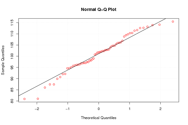
bitmap(file='test1.png')
myqqnorm <- qqnorm(x,col=2)
qqline(x)
grid()
dev.off()
load(file='createtable')
a<-table.start()
a<-table.row.start(a)
a<-table.element(a,'Percentiles - Ungrouped Data',9,TRUE)
a<-table.row.end(a)
a<-table.row.start(a)
a<-table.element(a,'p',1,TRUE)
a<-table.element(a,hyperlink('method_1.htm', 'Weighted Average at Xnp',''),1,TRUE)
a<-table.element(a,hyperlink('method_2.htm','Weighted Average at X(n+1)p',''),1,TRUE)
a<-table.element(a,hyperlink('method_3.htm','Empirical Distribution Function',''),1,TRUE)
a<-table.element(a,hyperlink('method_4.htm','Empirical Distribution Function - Averaging',''),1,TRUE)
a<-table.element(a,hyperlink('method_5.htm','Empirical Distribution Function - Interpolation',''),1,TRUE)
a<-table.element(a,hyperlink('method_6.htm','Closest Observation',''),1,TRUE)
a<-table.element(a,hyperlink('method_7.htm','True Basic - Statistics Graphics Toolkit',''),1,TRUE)
a<-table.element(a,hyperlink('method_8.htm','MS Excel (old versions)',''),1,TRUE)
a<-table.row.end(a)
for (perc in seq(mystart,99,mystep)) {
a<-table.row.start(a)
a<-table.element(a,round(perc/100,2),1,TRUE)
for (j in 1:8) {
a<-table.element(a,round(qval[perc,j],6))
}
a<-table.row.end(a)
}
a<-table.end(a)
table.save(a,file='mytable.tab')