Free Statistics
of Irreproducible Research!
Description of Statistical Computation | |||||||||||||||||||||||||||||||||||||
|---|---|---|---|---|---|---|---|---|---|---|---|---|---|---|---|---|---|---|---|---|---|---|---|---|---|---|---|---|---|---|---|---|---|---|---|---|---|
| Author's title | |||||||||||||||||||||||||||||||||||||
| Author | *The author of this computation has been verified* | ||||||||||||||||||||||||||||||||||||
| R Software Module | rwasp_boxcoxnorm.wasp | ||||||||||||||||||||||||||||||||||||
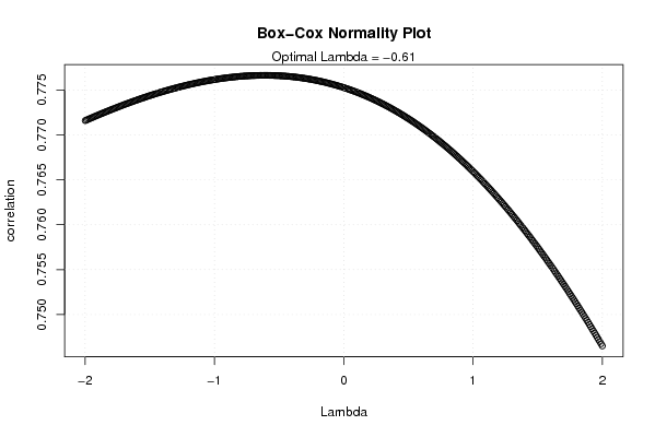
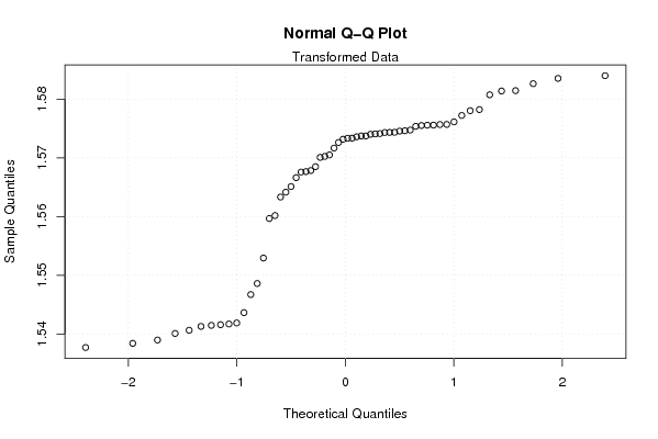
| Title produced by software | Box-Cox Normality Plot | ||||||||||||||||||||||||||||||||||||
| Date of computation | Sat, 29 Nov 2008 03:58:38 -0700 | ||||||||||||||||||||||||||||||||||||
| Cite this page as follows | Statistical Computations at FreeStatistics.org, Office for Research Development and Education, URL https://freestatistics.org/blog/index.php?v=date/2008/Nov/29/t1227956373q3999p1du0zmy3i.htm/, Retrieved Sat, 18 May 2024 19:41:10 +0000 | ||||||||||||||||||||||||||||||||||||
| Statistical Computations at FreeStatistics.org, Office for Research Development and Education, URL https://freestatistics.org/blog/index.php?pk=26196, Retrieved Sat, 18 May 2024 19:41:10 +0000 | |||||||||||||||||||||||||||||||||||||
| QR Codes: | |||||||||||||||||||||||||||||||||||||
|
| |||||||||||||||||||||||||||||||||||||
| Original text written by user: | |||||||||||||||||||||||||||||||||||||
| IsPrivate? | No (this computation is public) | ||||||||||||||||||||||||||||||||||||
| User-defined keywords | |||||||||||||||||||||||||||||||||||||
| Estimated Impact | 191 | ||||||||||||||||||||||||||||||||||||
Tree of Dependent Computations | |||||||||||||||||||||||||||||||||||||
| Family? (F = Feedback message, R = changed R code, M = changed R Module, P = changed Parameters, D = changed Data) | |||||||||||||||||||||||||||||||||||||
| - [Box-Cox Normality Plot] [Lambda 60] [2007-12-13 15:24:10] [ede03b06b9ae6a59763c2cc70a5f12fe] - PD [Box-Cox Normality Plot] [Box-Cox Normality...] [2008-11-29 10:58:38] [1b288879226ab9a3cab0c803857233cc] [Current] - D [Box-Cox Normality Plot] [Box-Cox Normality...] [2008-11-29 11:00:30] [8545382734d98368249ce527c6558129] - D [Box-Cox Normality Plot] [Box-Cox normality...] [2008-11-29 11:33:32] [8545382734d98368249ce527c6558129] - RMPD [Standard Deviation-Mean Plot] [SDMP (okt02-sept08)] [2008-11-29 11:37:20] [8545382734d98368249ce527c6558129] | |||||||||||||||||||||||||||||||||||||
| Feedback Forum | |||||||||||||||||||||||||||||||||||||
Post a new message | |||||||||||||||||||||||||||||||||||||
Dataset | |||||||||||||||||||||||||||||||||||||
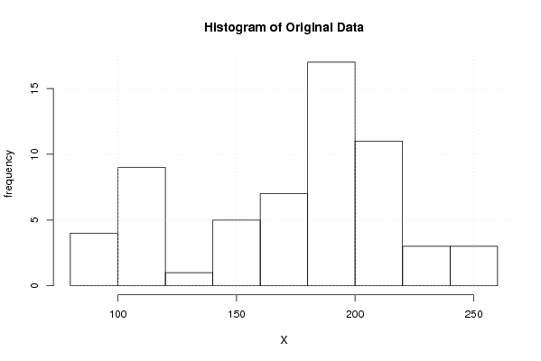
| Dataseries X: | |||||||||||||||||||||||||||||||||||||
95.4 101.2 101.5 101.9 101.7 100.1 97.4 96.5 99.2 102.2 105.3 111.1 114.9 124.5 142.2 159.7 165.2 198.6 207.8 219.6 239.6 235.3 218.5 213.8 205.5 198.4 198.5 190.2 180.7 193.6 192.8 195.5 197.2 196.9 178.9 172.4 156.4 143.7 153.6 168.8 185.8 199.9 205.4 197.5 199.6 200.5 193.7 179.6 169.1 169.8 195.5 194.8 204.5 203.8 204.8 204.9 240 248.3 258.4 254.9 | |||||||||||||||||||||||||||||||||||||
Tables (Output of Computation) | |||||||||||||||||||||||||||||||||||||
| |||||||||||||||||||||||||||||||||||||
Figures (Output of Computation) | |||||||||||||||||||||||||||||||||||||
Input Parameters & R Code | |||||||||||||||||||||||||||||||||||||
| Parameters (Session): | |||||||||||||||||||||||||||||||||||||
| Parameters (R input): | |||||||||||||||||||||||||||||||||||||
| R code (references can be found in the software module): | |||||||||||||||||||||||||||||||||||||
n <- length(x) | |||||||||||||||||||||||||||||||||||||