Free Statistics
of Irreproducible Research!
Description of Statistical Computation | |||||||||||||||||||||||||||||||||||||
|---|---|---|---|---|---|---|---|---|---|---|---|---|---|---|---|---|---|---|---|---|---|---|---|---|---|---|---|---|---|---|---|---|---|---|---|---|---|
| Author's title | |||||||||||||||||||||||||||||||||||||
| Author | *The author of this computation has been verified* | ||||||||||||||||||||||||||||||||||||
| R Software Module | rwasp_boxcoxnorm.wasp | ||||||||||||||||||||||||||||||||||||
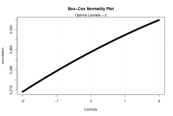
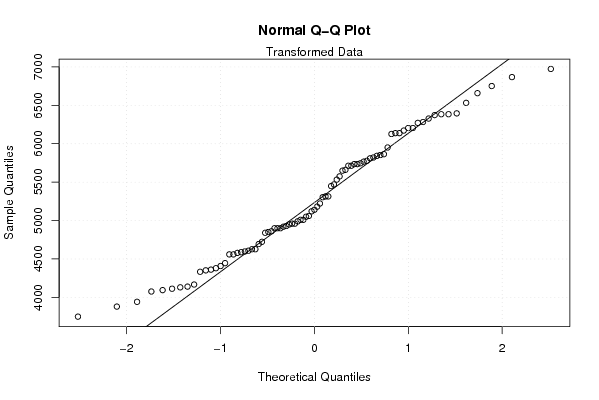
| Title produced by software | Box-Cox Normality Plot | ||||||||||||||||||||||||||||||||||||
| Date of computation | Tue, 11 Nov 2008 11:30:54 -0700 | ||||||||||||||||||||||||||||||||||||
| Cite this page as follows | Statistical Computations at FreeStatistics.org, Office for Research Development and Education, URL https://freestatistics.org/blog/index.php?v=date/2008/Nov/11/t1226428478mwxlazqqvln3hxj.htm/, Retrieved Sat, 18 May 2024 10:50:54 +0000 | ||||||||||||||||||||||||||||||||||||
| Statistical Computations at FreeStatistics.org, Office for Research Development and Education, URL https://freestatistics.org/blog/index.php?pk=23807, Retrieved Sat, 18 May 2024 10:50:54 +0000 | |||||||||||||||||||||||||||||||||||||
| QR Codes: | |||||||||||||||||||||||||||||||||||||
|
| |||||||||||||||||||||||||||||||||||||
| Original text written by user: | |||||||||||||||||||||||||||||||||||||
| IsPrivate? | No (this computation is public) | ||||||||||||||||||||||||||||||||||||
| User-defined keywords | Box-cox | ||||||||||||||||||||||||||||||||||||
| Estimated Impact | 181 | ||||||||||||||||||||||||||||||||||||
Tree of Dependent Computations | |||||||||||||||||||||||||||||||||||||
| Family? (F = Feedback message, R = changed R code, M = changed R Module, P = changed Parameters, D = changed Data) | |||||||||||||||||||||||||||||||||||||
| F [Box-Cox Normality Plot] [Box-cox normality...] [2008-11-11 18:30:54] [0cdfeda4aa2f9e551c2e529c44a404df] [Current] F D [Box-Cox Normality Plot] [box-cox normality ] [2008-11-12 20:05:49] [1eab65e90adf64584b8e6f0da23ff414] - R D [Box-Cox Normality Plot] [VAC Box-Cox Norma...] [2008-12-14 11:10:52] [379d6c32f73e3218fd773d79e4063d07] - D [Box-Cox Normality Plot] [VAC Box-Cox Norma...] [2008-12-23 14:54:04] [379d6c32f73e3218fd773d79e4063d07] - M D [Box-Cox Normality Plot] [Box-Cox Linearity...] [2010-01-23 19:00:37] [f1bd7399181c649098ca7b814ee0e027] - M D [Box-Cox Normality Plot] [Box-Cox Linearity...] [2010-01-23 18:59:13] [f1bd7399181c649098ca7b814ee0e027] - RMPD [Maximum-likelihood Fitting - Normal Distribution] [VAC Maximum Likeh...] [2008-12-14 11:15:17] [379d6c32f73e3218fd773d79e4063d07] - D [Maximum-likelihood Fitting - Normal Distribution] [VAC likelihood fi...] [2008-12-23 15:01:37] [379d6c32f73e3218fd773d79e4063d07] - M D [Maximum-likelihood Fitting - Normal Distribution] [Maximum-likelihoo...] [2010-01-23 19:03:12] [f1bd7399181c649098ca7b814ee0e027] - M [Maximum-likelihood Fitting - Normal Distribution] [Maximum-likelihoo...] [2010-01-23 19:01:52] [f1bd7399181c649098ca7b814ee0e027] - RM D [Kendall tau Correlation Matrix] [VAC kendall tau c...] [2008-12-14 11:50:35] [379d6c32f73e3218fd773d79e4063d07] - M [Kendall tau Correlation Matrix] [Kendall tau Corre...] [2010-01-23 19:04:12] [f1bd7399181c649098ca7b814ee0e027] - RM D [Kendall tau Rank Correlation] [VAC kendall tau c...] [2008-12-14 11:54:05] [379d6c32f73e3218fd773d79e4063d07] - M [Kendall tau Rank Correlation] [Kendall tau Corre...] [2010-01-23 19:07:20] [f1bd7399181c649098ca7b814ee0e027] | |||||||||||||||||||||||||||||||||||||
| Feedback Forum | |||||||||||||||||||||||||||||||||||||
Post a new message | |||||||||||||||||||||||||||||||||||||
Dataset | |||||||||||||||||||||||||||||||||||||
| Dataseries X: | |||||||||||||||||||||||||||||||||||||
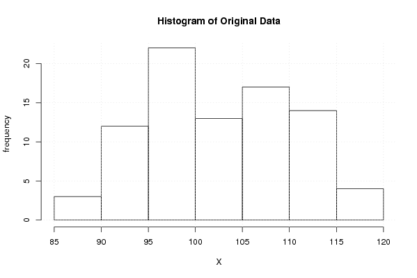
103,1 100,6 103,1 95,5 90,5 90,9 88,8 90,7 94,3 104,6 111,1 110,8 107,2 99 99 91 96,2 96,9 96,2 100,1 99 115,4 106,9 107,1 99,3 99,2 108,3 105,6 99,5 107,4 93,1 88,1 110,7 113,1 99,6 93,6 98,6 99,6 114,3 107,8 101,2 112,5 100,5 93,9 116,2 112 106,4 95,7 96 95,8 103 102,2 98,4 111,4 86,6 91,3 107,9 101,8 104,4 93,4 100,1 98,5 112,9 101,4 107,1 110,8 90,3 95,5 111,4 113 107,5 95,9 106,3 105,2 117,2 106,9 108,2 113 97,2 99,9 108,1 118,1 109,1 93,3 112,1 | |||||||||||||||||||||||||||||||||||||
Tables (Output of Computation) | |||||||||||||||||||||||||||||||||||||
| |||||||||||||||||||||||||||||||||||||
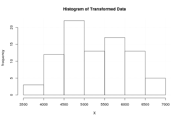
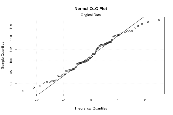
Figures (Output of Computation) | |||||||||||||||||||||||||||||||||||||
Input Parameters & R Code | |||||||||||||||||||||||||||||||||||||
| Parameters (Session): | |||||||||||||||||||||||||||||||||||||
| Parameters (R input): | |||||||||||||||||||||||||||||||||||||
| R code (references can be found in the software module): | |||||||||||||||||||||||||||||||||||||
n <- length(x) | |||||||||||||||||||||||||||||||||||||