Free Statistics
of Irreproducible Research!
Description of Statistical Computation | |||||||||||||||||||||
|---|---|---|---|---|---|---|---|---|---|---|---|---|---|---|---|---|---|---|---|---|---|
| Author's title | |||||||||||||||||||||
| Author | *The author of this computation has been verified* | ||||||||||||||||||||
| R Software Module | rwasp_meanplot.wasp | ||||||||||||||||||||
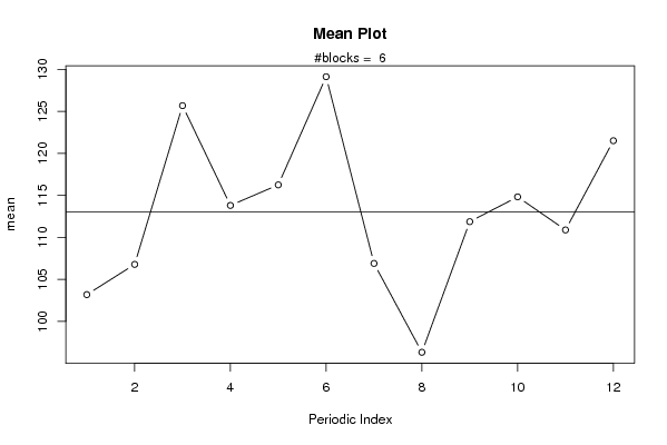
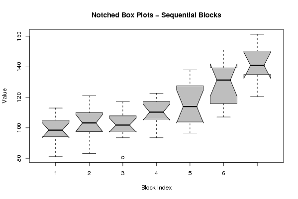
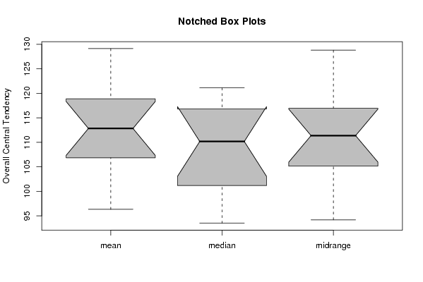
| Title produced by software | Mean Plot | ||||||||||||||||||||
| Date of computation | Fri, 26 Dec 2008 11:38:55 -0700 | ||||||||||||||||||||
| Cite this page as follows | Statistical Computations at FreeStatistics.org, Office for Research Development and Education, URL https://freestatistics.org/blog/index.php?v=date/2008/Dec/26/t1230316796bsu8gh63tyokh4c.htm/, Retrieved Sat, 18 May 2024 22:01:07 +0000 | ||||||||||||||||||||
| Statistical Computations at FreeStatistics.org, Office for Research Development and Education, URL https://freestatistics.org/blog/index.php?pk=36638, Retrieved Sat, 18 May 2024 22:01:07 +0000 | |||||||||||||||||||||
| QR Codes: | |||||||||||||||||||||
|
| |||||||||||||||||||||
| Original text written by user: | |||||||||||||||||||||
| IsPrivate? | No (this computation is public) | ||||||||||||||||||||
| User-defined keywords | Paper -seizoenaliteit - Mean plot - machines | ||||||||||||||||||||
| Estimated Impact | 216 | ||||||||||||||||||||
Tree of Dependent Computations | |||||||||||||||||||||
| Family? (F = Feedback message, R = changed R code, M = changed R Module, P = changed Parameters, D = changed Data) | |||||||||||||||||||||
| - [Mean Plot] [Paper - Mean plot...] [2007-11-27 18:19:55] [5343e105a400b9e32bf6f011133bbaf4] - D [Mean Plot] [Paper -seizoenali...] [2008-12-26 18:38:55] [3efbb18563b4564408d69b3c9a8e9a6e] [Current] | |||||||||||||||||||||
| Feedback Forum | |||||||||||||||||||||
Post a new message | |||||||||||||||||||||
Dataset | |||||||||||||||||||||
| Dataseries X: | |||||||||||||||||||||
93.5 94.7 112.9 99.2 105.6 113.0 83.1 81.1 96.9 104.3 97.7 102.6 89.9 96.0 112.7 107.1 106.2 121.0 101.2 83.2 105.1 113.3 99.1 100.3 93.5 98.8 106.2 98.3 102.1 117.1 101.5 80.5 105.9 109.5 97.2 114.5 93.5 100.9 121.1 116.5 109.3 118.1 108.3 105.4 116.2 111.2 105.8 122.7 99.5 107.9 124.6 115.0 110.3 132.7 99.7 96.5 118.7 112.9 130.5 137.9 115.0 116.8 140.9 120.7 134.2 147.3 112.4 107.1 128.4 137.7 135.0 151.0 137.4 132.4 161.3 139.8 146.0 154.6 142.1 120.5 | |||||||||||||||||||||
Tables (Output of Computation) | |||||||||||||||||||||
| |||||||||||||||||||||
Figures (Output of Computation) | |||||||||||||||||||||
Input Parameters & R Code | |||||||||||||||||||||
| Parameters (Session): | |||||||||||||||||||||
| par1 = 12 ; | |||||||||||||||||||||
| Parameters (R input): | |||||||||||||||||||||
| par1 = 12 ; | |||||||||||||||||||||
| R code (references can be found in the software module): | |||||||||||||||||||||
par1 <- as.numeric(par1) | |||||||||||||||||||||