Free Statistics
of Irreproducible Research!
Description of Statistical Computation | |||||||||||||||||||||||||||||||||||||||||||||
|---|---|---|---|---|---|---|---|---|---|---|---|---|---|---|---|---|---|---|---|---|---|---|---|---|---|---|---|---|---|---|---|---|---|---|---|---|---|---|---|---|---|---|---|---|---|
| Author's title | |||||||||||||||||||||||||||||||||||||||||||||
| Author | *The author of this computation has been verified* | ||||||||||||||||||||||||||||||||||||||||||||
| R Software Module | rwasp_boxcoxlin.wasp | ||||||||||||||||||||||||||||||||||||||||||||
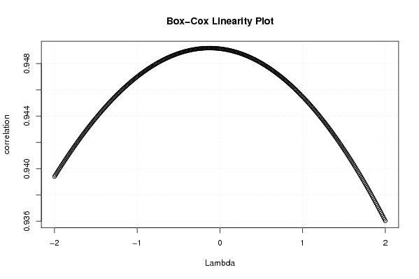
| Title produced by software | Box-Cox Linearity Plot | ||||||||||||||||||||||||||||||||||||||||||||
| Date of computation | Thu, 11 Dec 2008 16:59:13 -0700 | ||||||||||||||||||||||||||||||||||||||||||||
| Cite this page as follows | Statistical Computations at FreeStatistics.org, Office for Research Development and Education, URL https://freestatistics.org/blog/index.php?v=date/2008/Dec/12/t1229040002hf2q21nyxazw3nn.htm/, Retrieved Sat, 18 May 2024 05:42:22 +0000 | ||||||||||||||||||||||||||||||||||||||||||||
| Statistical Computations at FreeStatistics.org, Office for Research Development and Education, URL https://freestatistics.org/blog/index.php?pk=32482, Retrieved Sat, 18 May 2024 05:42:22 +0000 | |||||||||||||||||||||||||||||||||||||||||||||
| QR Codes: | |||||||||||||||||||||||||||||||||||||||||||||
|
| |||||||||||||||||||||||||||||||||||||||||||||
| Original text written by user: | |||||||||||||||||||||||||||||||||||||||||||||
| IsPrivate? | No (this computation is public) | ||||||||||||||||||||||||||||||||||||||||||||
| User-defined keywords | |||||||||||||||||||||||||||||||||||||||||||||
| Estimated Impact | 229 | ||||||||||||||||||||||||||||||||||||||||||||
Tree of Dependent Computations | |||||||||||||||||||||||||||||||||||||||||||||
| Family? (F = Feedback message, R = changed R code, M = changed R Module, P = changed Parameters, D = changed Data) | |||||||||||||||||||||||||||||||||||||||||||||
| - [Box-Cox Linearity Plot] [G6 paper box cox ...] [2007-11-25 10:03:41] [74be16979710d4c4e7c6647856088456] - D [Box-Cox Linearity Plot] [Box cox linearity...] [2008-12-11 23:53:24] [4ddbf81f78ea7c738951638c7e93f6ee] - D [Box-Cox Linearity Plot] [Box cox linearity...] [2008-12-11 23:56:02] [4ddbf81f78ea7c738951638c7e93f6ee] - D [Box-Cox Linearity Plot] [Box cox linearity...] [2008-12-11 23:59:13] [e8f764b122b426f433a1e1038b457077] [Current] | |||||||||||||||||||||||||||||||||||||||||||||
| Feedback Forum | |||||||||||||||||||||||||||||||||||||||||||||
Post a new message | |||||||||||||||||||||||||||||||||||||||||||||
Dataset | |||||||||||||||||||||||||||||||||||||||||||||
| Dataseries X: | |||||||||||||||||||||||||||||||||||||||||||||
9,4 9,5 9,1 9 9,3 9,9 9,8 9,4 8,3 8 8,5 10,4 11,1 10,9 9,9 9,2 9,2 9,5 9,6 9,5 9,1 8,9 9 10,1 10,3 10,2 9,6 9,2 9,3 9,4 9,4 9,2 9 9 9 9,8 10 9,9 9,3 9 9 9,1 9,1 9,1 9,2 8,8 8,3 8,4 8,1 7,8 7,9 7,9 8 7,9 7,5 7,2 6,9 6,6 6,7 7,3 | |||||||||||||||||||||||||||||||||||||||||||||
| Dataseries Y: | |||||||||||||||||||||||||||||||||||||||||||||
8.3 8.4 8.4 8.4 8.6 8.9 8.8 8.3 7.5 7.2 7.5 8.8 9.3 9.3 8.7 8.2 8.3 8.5 8.6 8.6 8.2 8.1 8 8.6 8.7 8.8 8.5 8.4 8.5 8.7 8.7 8.6 8.5 8.3 8.1 8.2 8.1 8.1 7.9 7.9 7.9 8 8 7.9 8 7.7 7.2 7.5 7.3 7 7 7 7.2 7.3 7.1 6.8 6.6 6.2 6.2 6.8 | |||||||||||||||||||||||||||||||||||||||||||||
Tables (Output of Computation) | |||||||||||||||||||||||||||||||||||||||||||||
| |||||||||||||||||||||||||||||||||||||||||||||
Figures (Output of Computation) | |||||||||||||||||||||||||||||||||||||||||||||
Input Parameters & R Code | |||||||||||||||||||||||||||||||||||||||||||||
| Parameters (Session): | |||||||||||||||||||||||||||||||||||||||||||||
| Parameters (R input): | |||||||||||||||||||||||||||||||||||||||||||||
| R code (references can be found in the software module): | |||||||||||||||||||||||||||||||||||||||||||||
n <- length(x) | |||||||||||||||||||||||||||||||||||||||||||||