Free Statistics
of Irreproducible Research!
Description of Statistical Computation | |||||||||||||||||||||||||||||||||||||||||||||
|---|---|---|---|---|---|---|---|---|---|---|---|---|---|---|---|---|---|---|---|---|---|---|---|---|---|---|---|---|---|---|---|---|---|---|---|---|---|---|---|---|---|---|---|---|---|
| Author's title | |||||||||||||||||||||||||||||||||||||||||||||
| Author | *The author of this computation has been verified* | ||||||||||||||||||||||||||||||||||||||||||||
| R Software Module | rwasp_boxcoxlin.wasp | ||||||||||||||||||||||||||||||||||||||||||||
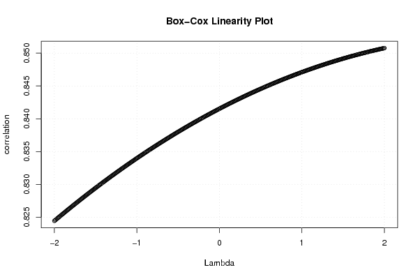
| Title produced by software | Box-Cox Linearity Plot | ||||||||||||||||||||||||||||||||||||||||||||
| Date of computation | Wed, 10 Dec 2008 08:02:30 -0700 | ||||||||||||||||||||||||||||||||||||||||||||
| Cite this page as follows | Statistical Computations at FreeStatistics.org, Office for Research Development and Education, URL https://freestatistics.org/blog/index.php?v=date/2008/Dec/10/t1228921490zedwrmbe39lu2ay.htm/, Retrieved Fri, 17 May 2024 12:54:53 +0000 | ||||||||||||||||||||||||||||||||||||||||||||
| Statistical Computations at FreeStatistics.org, Office for Research Development and Education, URL https://freestatistics.org/blog/index.php?pk=31990, Retrieved Fri, 17 May 2024 12:54:53 +0000 | |||||||||||||||||||||||||||||||||||||||||||||
| QR Codes: | |||||||||||||||||||||||||||||||||||||||||||||
|
| |||||||||||||||||||||||||||||||||||||||||||||
| Original text written by user: | |||||||||||||||||||||||||||||||||||||||||||||
| IsPrivate? | No (this computation is public) | ||||||||||||||||||||||||||||||||||||||||||||
| User-defined keywords | |||||||||||||||||||||||||||||||||||||||||||||
| Estimated Impact | 172 | ||||||||||||||||||||||||||||||||||||||||||||
Tree of Dependent Computations | |||||||||||||||||||||||||||||||||||||||||||||
| Family? (F = Feedback message, R = changed R code, M = changed R Module, P = changed Parameters, D = changed Data) | |||||||||||||||||||||||||||||||||||||||||||||
| - [Box-Cox Linearity Plot] [Paper G6 box cox ...] [2007-11-10 14:35:12] [70ea62757742573c580c86c5f8652367] - D [Box-Cox Linearity Plot] [Box-Cox Linearity...] [2008-12-10 15:02:30] [732c025e7dfb439ac3d0c7b7e70fa7a1] [Current] - D [Box-Cox Linearity Plot] [Box-Cox Linearity...] [2008-12-18 13:19:27] [7506b5e9e41ec66c6657f4234f97306e] | |||||||||||||||||||||||||||||||||||||||||||||
| Feedback Forum | |||||||||||||||||||||||||||||||||||||||||||||
Post a new message | |||||||||||||||||||||||||||||||||||||||||||||
Dataset | |||||||||||||||||||||||||||||||||||||||||||||
| Dataseries X: | |||||||||||||||||||||||||||||||||||||||||||||
103,2 106,9 118,6 111,9 119,0 116,3 116,2 115,6 107,5 116,8 124,1 115,0 105,3 104,1 119,6 112,2 109,6 121,8 108,8 111,5 108,5 115,4 119,3 116,5 101,9 96,6 116,6 112,5 103,7 118,5 105,0 105,0 109,1 112,6 108,2 114,4 95,9 90,8 115,0 99,8 103,0 108,4 99,2 100,6 107,1 107,0 111,9 115,6 97,7 97,3 111,8 99,3 104,6 113,3 98,7 98,2 102,5 100,8 111,4 108,9 90,4 94,6 104,3 99,0 103,0 105,1 98,9 101,0 96,5 102,8 112,3 106,5 91,9 92,7 104,2 101,7 102,8 105,6 96,9 97,6 93,7 102,1 106,6 100,2 92,0 86,8 104,8 100,0 96,8 110,6 100,7 101,5 | |||||||||||||||||||||||||||||||||||||||||||||
| Dataseries Y: | |||||||||||||||||||||||||||||||||||||||||||||
18 562,2 23 184,8 22 925,8 21 490,2 23 243,2 21 688,7 21 423,1 21 211,2 17 877,4 20 664,3 22 160,0 19 813,6 17 735,4 19 640,2 20 844,4 19 823,1 18 594,6 21 350,6 18 574,1 18 924,2 17 343,4 19 961,2 19 932,1 19 464,6 16 165,4 17 574,9 19 795,4 19 439,5 17 170,0 21 072,4 17 751,8 17 515,5 18 040,3 19 090,1 17 746,5 19 202,1 15 141,6 16 258,1 18 586,5 17 209,4 17 838,7 19 123,5 16 583,6 15 991,2 16 704,4 17 420,4 17 872,0 17 823,2 13 866,5 15 912,8 17 870,5 15 420,3 16 379,4 17 903,9 15 305,8 14 583,3 14 861,0 14 968,9 16 726,5 16 283,6 11 703,7 15 101,8 15 469,7 14 956,9 15 370,6 15 998,1 14 725,1 14 768,9 13 659,6 15 070,3 16 943,0 15 761,3 12 083,0 15 023,6 15 106,5 15 498,6 15 258,9 15 859,4 14 205,3 14 291,1 12 875,1 14 755,3 15 873,2 14 803,0 12 520,2 14 568,3 15 644,8 15 454,9 14 254,0 16 754,8 14 944,2 15 044,5 | |||||||||||||||||||||||||||||||||||||||||||||
Tables (Output of Computation) | |||||||||||||||||||||||||||||||||||||||||||||
| |||||||||||||||||||||||||||||||||||||||||||||
Figures (Output of Computation) | |||||||||||||||||||||||||||||||||||||||||||||
Input Parameters & R Code | |||||||||||||||||||||||||||||||||||||||||||||
| Parameters (Session): | |||||||||||||||||||||||||||||||||||||||||||||
| Parameters (R input): | |||||||||||||||||||||||||||||||||||||||||||||
| R code (references can be found in the software module): | |||||||||||||||||||||||||||||||||||||||||||||
n <- length(x) | |||||||||||||||||||||||||||||||||||||||||||||