| Multiple Linear Regression - Estimated Regression Equation |
| DE[t] = + 33.3249 + 0.491587`Solids,`[t] + 0.00123242`Osmo,`[t] -0.0262518t + e[t] |
| Multiple Linear Regression - Ordinary Least Squares | |||||
| Variable | Parameter | S.D. | T-STAT H0: parameter = 0 | 2-tail p-value | 1-tail p-value |
| (Intercept) | +33.33 | 4.257 | +7.8270e+00 | 2.042e-08 | 1.021e-08 |
| `Solids,` | +0.4916 | 0.6357 | +7.7330e-01 | 0.446 | 0.223 |
| `Osmo,` | +0.001232 | 0.01534 | +8.0320e-02 | 0.9366 | 0.4683 |
| t | -0.02625 | 0.0237 | -1.1080e+00 | 0.2777 | 0.1388 |
| Multiple Linear Regression - Regression Statistics | |
| Multiple R | 0.5711 |
| R-squared | 0.3262 |
| Adjusted R-squared | 0.2513 |
| F-TEST (value) | 4.357 |
| F-TEST (DF numerator) | 3 |
| F-TEST (DF denominator) | 27 |
| p-value | 0.01258 |
| Multiple Linear Regression - Residual Statistics | |
| Residual Standard Deviation | 1.172 |
| Sum Squared Residuals | 37.07 |
| Menu of Residual Diagnostics | |
| Description | Link |
| Histogram | Compute |
| Central Tendency | Compute |
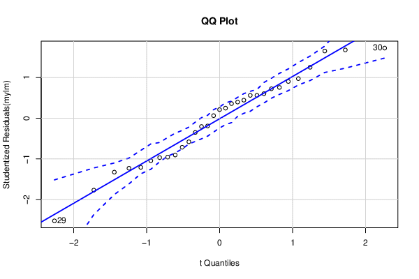
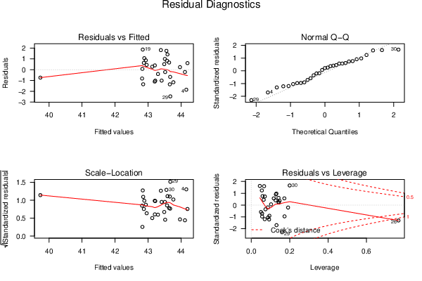
| QQ Plot | Compute |
| Kernel Density Plot | Compute |
| Skewness/Kurtosis Test | Compute |
| Skewness-Kurtosis Plot | Compute |
| Harrell-Davis Plot | Compute |
| Bootstrap Plot -- Central Tendency | Compute |
| Blocked Bootstrap Plot -- Central Tendency | Compute |
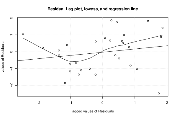
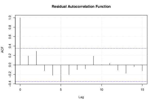
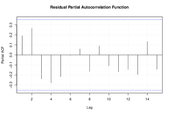
| (Partial) Autocorrelation Plot | Compute |
| Spectral Analysis | Compute |
| Tukey lambda PPCC Plot | Compute |
| Box-Cox Normality Plot | Compute |
| Summary Statistics | Compute |
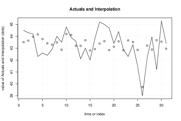
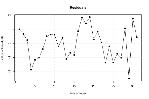
| Multiple Linear Regression - Actuals, Interpolation, and Residuals | |||
| Time or Index | Actuals | Interpolation Forecast | Residuals Prediction Error |
| 1 | 44.5 | 43.51 | 0.9915 |
| 2 | 44.3 | 43.64 | 0.6628 |
| 3 | 44.2 | 43.97 | 0.2339 |
| 4 | 42.3 | 44.16 | -1.858 |
| 5 | 42.6 | 43.77 | -1.166 |
| 6 | 42.4 | 43.41 | -1.01 |
| 7 | 42.9 | 43.3 | -0.4006 |
| 8 | 44 | 43.49 | 0.5105 |
| 9 | 43.5 | 42.87 | 0.6269 |
| 10 | 44.8 | 44.19 | 0.6069 |
| 11 | 43.9 | 44.12 | -0.2163 |
| 12 | 43.6 | 43.2 | 0.3951 |
| 13 | 42.1 | 43.2 | -1.102 |
| 14 | 43 | 43.67 | -0.6688 |
| 15 | 42 | 42.82 | -0.8189 |
| 16 | 43.8 | 42.93 | 0.8672 |
| 17 | 45.2 | 43.39 | 1.813 |
| 18 | 45 | 43.59 | 1.412 |
| 19 | 44.7 | 42.84 | 1.861 |
| 20 | 43.4 | 43.13 | 0.2736 |
| 21 | 44.4 | 43.57 | 0.8252 |
| 22 | 42.9 | 42.83 | 0.07178 |
| 23 | 42.3 | 43.66 | -1.359 |
| 24 | 43.3 | 43.52 | -0.2181 |
| 25 | 41.5 | 42.85 | -1.353 |
| 26 | 39 | 39.74 | -0.7385 |
| 27 | 42.2 | 43.22 | -1.018 |
| 28 | 43.95 | 42.89 | 1.064 |
| 29 | 41.2 | 43.67 | -2.473 |
| 30 | 45.3 | 43.56 | 1.744 |
| 31 | 43.4 | 42.96 | 0.4418 |
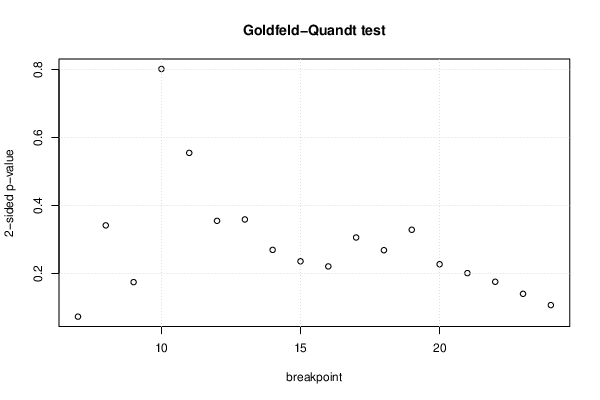
| Goldfeld-Quandt test for Heteroskedasticity | |||
| p-values | Alternative Hypothesis | ||
| breakpoint index | greater | 2-sided | less |
| 7 | 0.03674 | 0.07347 | 0.9633 |
| 8 | 0.1709 | 0.3418 | 0.8291 |
| 9 | 0.08745 | 0.1749 | 0.9126 |
| 10 | 0.4008 | 0.8016 | 0.5992 |
| 11 | 0.2774 | 0.5548 | 0.7226 |
| 12 | 0.1776 | 0.3551 | 0.8224 |
| 13 | 0.1796 | 0.3592 | 0.8204 |
| 14 | 0.1349 | 0.2698 | 0.8651 |
| 15 | 0.1181 | 0.2362 | 0.8819 |
| 16 | 0.1106 | 0.2212 | 0.8894 |
| 17 | 0.1531 | 0.3062 | 0.8469 |
| 18 | 0.1344 | 0.2688 | 0.8656 |
| 19 | 0.1644 | 0.3288 | 0.8356 |
| 20 | 0.1137 | 0.2275 | 0.8863 |
| 21 | 0.1007 | 0.2014 | 0.8993 |
| 22 | 0.08797 | 0.1759 | 0.912 |
| 23 | 0.0703 | 0.1406 | 0.9297 |
| 24 | 0.05371 | 0.1074 | 0.9463 |
| Meta Analysis of Goldfeld-Quandt test for Heteroskedasticity | |||
| Description | # significant tests | % significant tests | OK/NOK |
| 1% type I error level | 0 | 0 | OK |
| 5% type I error level | 0 | 0 | OK |
| 10% type I error level | 1 | 0.0555556 | OK |
| Ramsey RESET F-Test for powers (2 and 3) of fitted values |
> reset_test_fitted RESET test data: mylm RESET = 0.90321, df1 = 2, df2 = 25, p-value = 0.4181 |
| Ramsey RESET F-Test for powers (2 and 3) of regressors |
> reset_test_regressors RESET test data: mylm RESET = 0.67924, df1 = 6, df2 = 21, p-value = 0.668 |
| Ramsey RESET F-Test for powers (2 and 3) of principal components |
> reset_test_principal_components RESET test data: mylm RESET = 0.98183, df1 = 2, df2 = 25, p-value = 0.3886 |
| Variance Inflation Factors (Multicollinearity) |
> vif `Solids,` `Osmo,` t 15.466179 15.411955 1.014185 |