| Multiple Linear Regression - Estimated Regression Equation |
| a[t] = + 51.5827 + 0.0757179b[t] -3.46203c[t] + e[t] |
| Multiple Linear Regression - Ordinary Least Squares | |||||
| Variable | Parameter | S.D. | T-STAT H0: parameter = 0 | 2-tail p-value | 1-tail p-value |
| (Intercept) | +51.58 | 8.825 | +5.8450e+00 | 2.778e-06 | 1.389e-06 |
| b | +0.07572 | 0.05531 | +1.3690e+00 | 0.1819 | 0.09095 |
| c | -3.462 | 0.957 | -3.6180e+00 | 0.00116 | 0.0005798 |
| Multiple Linear Regression - Regression Statistics | |
| Multiple R | 0.5699 |
| R-squared | 0.3248 |
| Adjusted R-squared | 0.2766 |
| F-TEST (value) | 6.734 |
| F-TEST (DF numerator) | 2 |
| F-TEST (DF denominator) | 28 |
| p-value | 0.004094 |
| Multiple Linear Regression - Residual Statistics | |
| Residual Standard Deviation | 2.159 |
| Sum Squared Residuals | 130.5 |
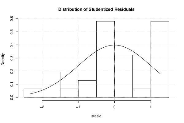
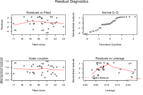
| Menu of Residual Diagnostics | |
| Description | Link |
| Histogram | Compute |
| Central Tendency | Compute |
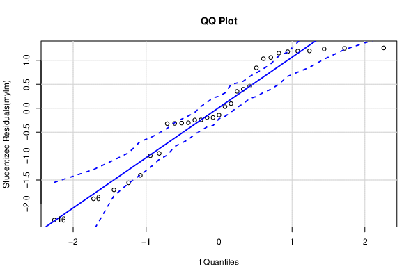
| QQ Plot | Compute |
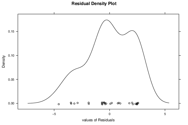
| Kernel Density Plot | Compute |
| Skewness/Kurtosis Test | Compute |
| Skewness-Kurtosis Plot | Compute |
| Harrell-Davis Plot | Compute |
| Bootstrap Plot -- Central Tendency | Compute |
| Blocked Bootstrap Plot -- Central Tendency | Compute |
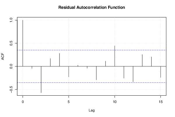
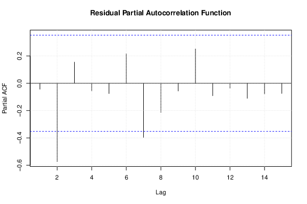
| (Partial) Autocorrelation Plot | Compute |
| Spectral Analysis | Compute |
| Tukey lambda PPCC Plot | Compute |
| Box-Cox Normality Plot | Compute |
| Summary Statistics | Compute |
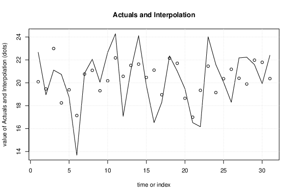
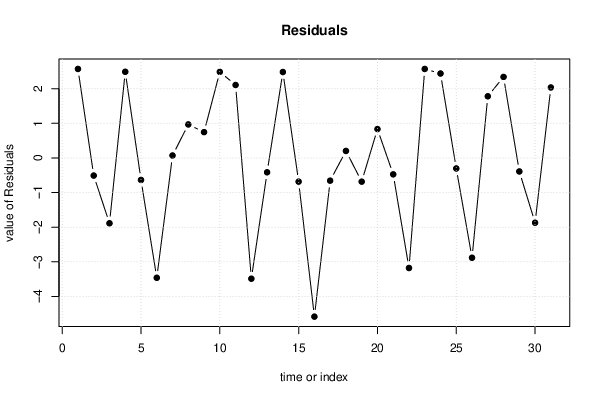
| Multiple Linear Regression - Actuals, Interpolation, and Residuals | |||
| Time or Index | Actuals | Interpolation Forecast | Residuals Prediction Error |
| 1 | 22.66 | 20.09 | 2.57 |
| 2 | 18.95 | 19.46 | -0.5094 |
| 3 | 21.11 | 22.99 | -1.888 |
| 4 | 20.73 | 18.24 | 2.488 |
| 5 | 18.75 | 19.39 | -0.6362 |
| 6 | 13.68 | 17.14 | -3.462 |
| 7 | 20.83 | 20.76 | 0.06984 |
| 8 | 22.06 | 21.09 | 0.9679 |
| 9 | 20.05 | 19.31 | 0.745 |
| 10 | 22.66 | 20.17 | 2.485 |
| 11 | 24.28 | 22.17 | 2.107 |
| 12 | 17.07 | 20.56 | -3.489 |
| 13 | 21.11 | 21.52 | -0.4148 |
| 14 | 24.11 | 21.63 | 2.482 |
| 15 | 19.78 | 20.46 | -0.685 |
| 16 | 16.52 | 21.11 | -4.585 |
| 17 | 18.3 | 18.96 | -0.6568 |
| 18 | 22.35 | 22.14 | 0.2023 |
| 19 | 21.02 | 21.7 | -0.6856 |
| 20 | 19.48 | 18.64 | 0.8339 |
| 21 | 16.52 | 16.99 | -0.4744 |
| 22 | 16.16 | 19.34 | -3.179 |
| 23 | 24.02 | 21.45 | 2.571 |
| 24 | 21.59 | 19.15 | 2.438 |
| 25 | 20.05 | 20.36 | -0.3048 |
| 26 | 18.3 | 21.18 | -2.884 |
| 27 | 22.18 | 20.39 | 1.781 |
| 28 | 22.23 | 19.89 | 2.341 |
| 29 | 21.59 | 21.98 | -0.3906 |
| 30 | 19.92 | 21.79 | -1.872 |
| 31 | 22.4 | 20.37 | 2.035 |
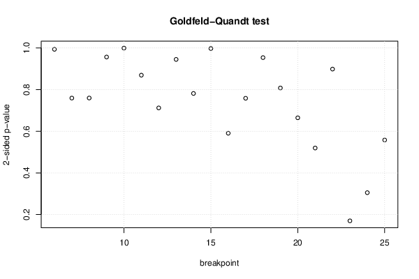
| Goldfeld-Quandt test for Heteroskedasticity | |||
| p-values | Alternative Hypothesis | ||
| breakpoint index | greater | 2-sided | less |
| 6 | 0.4969 | 0.9938 | 0.5031 |
| 7 | 0.6202 | 0.7595 | 0.3798 |
| 8 | 0.6201 | 0.7597 | 0.3799 |
| 9 | 0.5217 | 0.9567 | 0.4783 |
| 10 | 0.4998 | 0.9996 | 0.5002 |
| 11 | 0.4347 | 0.8694 | 0.5653 |
| 12 | 0.6439 | 0.7122 | 0.3561 |
| 13 | 0.5274 | 0.9452 | 0.4726 |
| 14 | 0.6092 | 0.7817 | 0.3908 |
| 15 | 0.4988 | 0.9976 | 0.5012 |
| 16 | 0.7047 | 0.5906 | 0.2953 |
| 17 | 0.6207 | 0.7586 | 0.3793 |
| 18 | 0.5231 | 0.9539 | 0.4769 |
| 19 | 0.404 | 0.808 | 0.596 |
| 20 | 0.3324 | 0.6647 | 0.6676 |
| 21 | 0.2598 | 0.5196 | 0.7402 |
| 22 | 0.5506 | 0.8987 | 0.4494 |
| 23 | 0.9152 | 0.1697 | 0.08485 |
| 24 | 0.8474 | 0.3051 | 0.1526 |
| 25 | 0.721 | 0.5581 | 0.279 |
| Meta Analysis of Goldfeld-Quandt test for Heteroskedasticity | |||
| Description | # significant tests | % significant tests | OK/NOK |
| 1% type I error level | 0 | 0 | OK |
| 5% type I error level | 0 | 0 | OK |
| 10% type I error level | 0 | 0 | OK |
| Ramsey RESET F-Test for powers (2 and 3) of fitted values |
> reset_test_fitted RESET test data: mylm RESET = 0.89829, df1 = 2, df2 = 26, p-value = 0.4195 |
| Ramsey RESET F-Test for powers (2 and 3) of regressors |
> reset_test_regressors RESET test data: mylm RESET = 0.21554, df1 = 4, df2 = 24, p-value = 0.9272 |
| Ramsey RESET F-Test for powers (2 and 3) of principal components |
> reset_test_principal_components RESET test data: mylm RESET = 0.29568, df1 = 2, df2 = 26, p-value = 0.7465 |
| Variance Inflation Factors (Multicollinearity) |
> vif
       b        c
1.046821 1.046821
|