Repository of Reproducible Computations

Free Statistics

of Irreproducible Research!

Author's title

Author

*Unverified author*

R Software Module

rwasp_boxcoxnorm.wasp

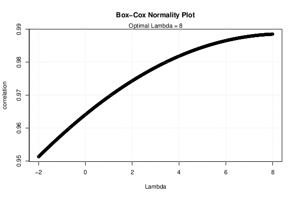
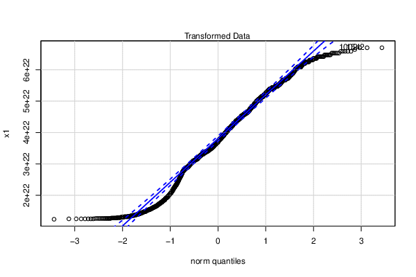
Title produced by software

Box-Cox Normality Plot

Date of computation

Tue, 06 Apr 2021 21:46:55 +0200

Cite this page as follows

Statistical Computations at FreeStatistics.org, Office for Research Development and Education, URL https://freestatistics.org/blog/index.php?v=date/2021/Apr/06/t1617738543h55xg4secz5rsn8.htm/, Retrieved Sat, 04 May 2024 00:39:04 +0200

Statistical Computations at FreeStatistics.org, Office for Research Development and Education, URL https://freestatistics.org/blog/index.php?pk=, Retrieved Sat, 04 May 2024 00:39:04 +0200

QR Codes:

Paste this QR Code to cite your computation.

Original text written by user:

IsPrivate?

This computation is private

User-defined keywords

Estimated Impact

Dataseries X:

Download CSV

Histogram

Boxplots

Summary of computational transaction
Raw Input	view raw input (R code)
Raw Output	view raw output of R engine
Computing time	2 seconds
R Server	Big Analytics Cloud Computing Center

\begin{tabular}{lllllllll}
\hline
Summary of computational transaction \tabularnewline
Raw Input view raw input (R code)  \tabularnewline
Raw Outputview raw output of R engine  \tabularnewline
Computing time2 seconds \tabularnewline
R ServerBig Analytics Cloud Computing Center \tabularnewline
\hline
\end{tabular}
%Source: https://freestatistics.org/blog/index.php?pk=&T=0

[TABLE]
[ROW]

Summary of computational transaction[/C][/ROW] [ROW]

Raw Input[/C]

view raw input (R code) [/C][/ROW] [ROW]

Raw Output[/C]

view raw output of R engine [/C][/ROW] [ROW]

Computing time[/C]

2 seconds[/C][/ROW] [ROW]

R Server[/C]

Big Analytics Cloud Computing Center[/C][/ROW] [/TABLE] Source: https://freestatistics.org/blog/index.php?pk=&T=0

Globally Unique Identifier (entire table): ba.freestatistics.org/blog/index.php?pk=&T=0

As an alternative you can also use a QR Code:

The GUIDs for individual cells are displayed in the table below:

Summary of computational transaction
Raw Input	view raw input (R code)
Raw Output	view raw output of R engine
Computing time	2 seconds
R Server	Big Analytics Cloud Computing Center

Box-Cox Normality Plot
# observations x	1677
maximum correlation	0.988512059760626
optimal lambda	8
transformation formula	for all lambda <> 0 : T(Y) = (Y^lambda - 1) / lambda

\begin{tabular}{lllllllll}
\hline
Box-Cox Normality Plot \tabularnewline
# observations x & 1677 \tabularnewline
maximum correlation & 0.988512059760626 \tabularnewline
optimal lambda & 8 \tabularnewline
transformation formula & for all lambda <> 0 : T(Y) = (Y^lambda - 1) / lambda \tabularnewline
\hline
\end{tabular}
%Source: https://freestatistics.org/blog/index.php?pk=&T=1

[TABLE]
[ROW][C]Box-Cox Normality Plot[/C][/ROW]
[ROW][C]# observations x[/C][C]1677[/C][/ROW]
[ROW][C]maximum correlation[/C][C]0.988512059760626[/C][/ROW]
[ROW][C]optimal lambda[/C][C]8[/C][/ROW]
[ROW][C]transformation formula[/C][C]for all lambda <> 0 : T(Y) = (Y^lambda - 1) / lambda[/C][/ROW]
[/TABLE]
Source: https://freestatistics.org/blog/index.php?pk=&T=1

Globally Unique Identifier (entire table): ba.freestatistics.org/blog/index.php?pk=&T=1

As an alternative you can also use a QR Code:

The GUIDs for individual cells are displayed in the table below:

Box-Cox Normality Plot
# observations x	1677
maximum correlation	0.988512059760626
optimal lambda	8
transformation formula	for all lambda <> 0 : T(Y) = (Y^lambda - 1) / lambda

Maximum Likelihood Estimation of Lambda

> summary(mypT)
bcPower Transformation to Normality 
  Est Power Rounded Pwr Wald Lwr Bnd Wald Upr Bnd
x    7.0691        7.07       6.1439       7.9943
Likelihood ratio test that transformation parameter is equal to 0
 (log transformation)
                           LRT df       pval
LR test, lambda = (0) 236.7434  1 < 2.22e-16
Likelihood ratio test that no transformation is needed
                           LRT df       pval
LR test, lambda = (1) 173.4809  1 < 2.22e-16

\begin{tabular}{lllllllll}
\hline
Maximum Likelihood Estimation of Lambda \tabularnewline
> summary(mypT)
bcPower Transformation to Normality 
  Est Power Rounded Pwr Wald Lwr Bnd Wald Upr Bnd
x    7.0691        7.07       6.1439       7.9943
Likelihood ratio test that transformation parameter is equal to 0
 (log transformation)
                           LRT df       pval
LR test, lambda = (0) 236.7434  1 < 2.22e-16
Likelihood ratio test that no transformation is needed
                           LRT df       pval
LR test, lambda = (1) 173.4809  1 < 2.22e-16
 \tabularnewline
\hline
\end{tabular}
%Source: https://freestatistics.org/blog/index.php?pk=&T=2

[TABLE]
[ROW][C]Maximum Likelihood Estimation of Lambda[/C][/ROW]
[ROW][C]> summary(mypT)
bcPower Transformation to Normality 
  Est Power Rounded Pwr Wald Lwr Bnd Wald Upr Bnd
x    7.0691        7.07       6.1439       7.9943
Likelihood ratio test that transformation parameter is equal to 0
 (log transformation)
                           LRT df       pval
LR test, lambda = (0) 236.7434  1 < 2.22e-16
Likelihood ratio test that no transformation is needed
                           LRT df       pval
LR test, lambda = (1) 173.4809  1 < 2.22e-16
[/C][/ROW]
[/TABLE]
Source: https://freestatistics.org/blog/index.php?pk=&T=2

Globally Unique Identifier (entire table): ba.freestatistics.org/blog/index.php?pk=&T=2

As an alternative you can also use a QR Code:

The GUIDs for individual cells are displayed in the table below:

Maximum Likelihood Estimation of Lambda

> summary(mypT)
bcPower Transformation to Normality 
  Est Power Rounded Pwr Wald Lwr Bnd Wald Upr Bnd
x    7.0691        7.07       6.1439       7.9943
Likelihood ratio test that transformation parameter is equal to 0
 (log transformation)
                           LRT df       pval
LR test, lambda = (0) 236.7434  1 < 2.22e-16
Likelihood ratio test that no transformation is needed
                           LRT df       pval
LR test, lambda = (1) 173.4809  1 < 2.22e-16

Figure 1

PNG link

Postscript link

PDF link

Figure 2

PNG link

Postscript link

PDF link

Figure 3

PNG link

Postscript link

PDF link

Figure 4

PNG link

Postscript link

PDF link

Figure 5

PNG link

Postscript link

PDF link

Parameters (Session):

par1 = Full Box-Cox transform ; par2 = -2 ; par3 = 8 ; par4 = 0 ; par5 = No ;

Parameters (R input):

par1 = Full Box-Cox transform ; par2 = -2 ; par3 = 8 ; par4 = 0 ; par5 = No ;

R code (references can be found in the software module):

par5 <- 'No'
par4 <- '0'
par3 <- '2'
par2 <- '-2'
par1 <- 'Full Box-Cox transform'
library(car)
par2 <- abs(as.numeric(par2)*100)
par3 <- as.numeric(par3)*100
if(par4=='') par4 <- 0
par4 <- as.numeric(par4)
numlam <- par2 + par3 + 1
x <- x + par4
n <- length(x)
c <- array(NA,dim=c(numlam))
l <- array(NA,dim=c(numlam))
mx <- -1
mxli <- -999
for (i in 1:numlam)
{
l[i] <- (i-par2-1)/100
if (l[i] != 0)
{
if (par1 == 'Full Box-Cox transform') x1 <- (x^l[i] - 1) / l[i]
if (par1 == 'Simple Box-Cox transform') x1 <- x^l[i]
} else {
x1 <- log(x)
}
c[i] <- cor(qnorm(ppoints(x), mean=0, sd=1),sort(x1))
if (mx < c[i])
{
mx <- c[i]
mxli <- l[i]
x1.best <- x1
}
}
print(c)
print(mx)
print(mxli)
print(x1.best)
if (mxli != 0)
{
if (par1 == 'Full Box-Cox transform') x1 <- (x^mxli - 1) / mxli
if (par1 == 'Simple Box-Cox transform') x1 <- x^mxli
} else {
x1 <- log(x)
}
mypT <- powerTransform(x)
summary(mypT)
bitmap(file='test1.png')
plot(l,c,main='Box-Cox Normality Plot', xlab='Lambda',ylab='correlation')
mtext(paste('Optimal Lambda =',mxli))
grid()
dev.off()
bitmap(file='test2.png')
hist(x,main='Histogram of Original Data',xlab='X',ylab='frequency')
grid()
dev.off()
bitmap(file='test3.png')
hist(x1,main='Histogram of Transformed Data', xlab='X',ylab='frequency')
grid()
dev.off()
bitmap(file='test4.png')
qqPlot(x)
grid()
mtext('Original Data')
dev.off()
bitmap(file='test5.png')
qqPlot(x1)
grid()
mtext('Transformed Data')
dev.off()
load(file='createtable')
a<-table.start()
a<-table.row.start(a)
a<-table.element(a,'Box-Cox Normality Plot',2,TRUE)
a<-table.row.end(a)
a<-table.row.start(a)
a<-table.element(a,'# observations x',header=TRUE)
a<-table.element(a,n)
a<-table.row.end(a)
a<-table.row.start(a)
a<-table.element(a,'maximum correlation',header=TRUE)
a<-table.element(a,mx)
a<-table.row.end(a)
a<-table.row.start(a)
a<-table.element(a,'optimal lambda',header=TRUE)
a<-table.element(a,mxli)
a<-table.row.end(a)
a<-table.row.start(a)
a<-table.element(a,'transformation formula',header=TRUE)
if (par1 == 'Full Box-Cox transform') {
a<-table.element(a,'for all lambda <> 0 : T(Y) = (Y^lambda - 1) / lambda')
} else {
a<-table.element(a,'for all lambda <> 0 : T(Y) = Y^lambda')
}
a<-table.row.end(a)
if(mx<0) {
a<-table.row.start(a)
a<-table.element(a,'Warning: maximum correlation is negative! The Box-Cox transformation must not be used.',2)
a<-table.row.end(a)
}
a<-table.end(a)
table.save(a,file='mytable.tab')
if(par5=='Yes') {
a<-table.start()
a<-table.row.start(a)
a<-table.element(a,'Obs.',header=T)
a<-table.element(a,'Original',header=T)
a<-table.element(a,'Transformed',header=T)
a<-table.row.end(a)
for (i in 1:n) {
a<-table.row.start(a)
a<-table.element(a,i)
a<-table.element(a,x[i])
a<-table.element(a,x1.best[i])
a<-table.row.end(a)
}
a<-table.end(a)
table.save(a,file='mytable1.tab')
}
a<-table.start()
a<-table.row.start(a)
a<-table.element(a,'Maximum Likelihood Estimation of Lambda',1,TRUE)
a<-table.row.end(a)
a<-table.row.start(a)
a<-table.element(a,paste('',RC.texteval('summary(mypT)'),'
',sep=''))
a<-table.row.end(a)
a<-table.end(a)
table.save(a,file='mytable3.tab')

Free Statistics

Description of Statistical Computation

Tree of Dependent Computations

Dataset

Tables (Output of Computation)

Figures (Output of Computation)

Input Parameters & R Code