| Multiple Linear Regression - Estimated Regression Equation |
| TVDCSUM[t] = + 2.78913 + 0.687324`SK/EOU1`[t] + 0.893553`SK/EOU2`[t] + 0.604347`SK/EOU4`[t] + 0.0329226IKSUM[t] + 0.512012GW1[t] + 0.560009GW2[t] + 0.0616104ECSUM[t] + e[t] |
| Multiple Linear Regression - Ordinary Least Squares | |||||
| Variable | Parameter | S.D. | T-STAT H0: parameter = 0 | 2-tail p-value | 1-tail p-value |
| (Intercept) | +2.789 | 2.026 | +1.3770e+00 | 0.1725 | 0.08623 |
| `SK/EOU1` | +0.6873 | 0.2003 | +3.4310e+00 | 0.0009535 | 0.0004768 |
| `SK/EOU2` | +0.8935 | 0.242 | +3.6920e+00 | 0.0004046 | 0.0002023 |
| `SK/EOU4` | +0.6044 | 0.2786 | +2.1700e+00 | 0.03301 | 0.01651 |
| IKSUM | +0.03292 | 0.08156 | +4.0370e-01 | 0.6875 | 0.3438 |
| GW1 | +0.512 | 0.2376 | +2.1550e+00 | 0.03415 | 0.01707 |
| GW2 | +0.56 | 0.1574 | +3.5570e+00 | 0.0006329 | 0.0003165 |
| ECSUM | +0.06161 | 0.05167 | +1.1920e+00 | 0.2367 | 0.1183 |
| Multiple Linear Regression - Regression Statistics | |
| Multiple R | 0.704 |
| R-squared | 0.4956 |
| Adjusted R-squared | 0.4515 |
| F-TEST (value) | 11.23 |
| F-TEST (DF numerator) | 7 |
| F-TEST (DF denominator) | 80 |
| p-value | 8.054e-10 |
| Multiple Linear Regression - Residual Statistics | |
| Residual Standard Deviation | 1.332 |
| Sum Squared Residuals | 142 |
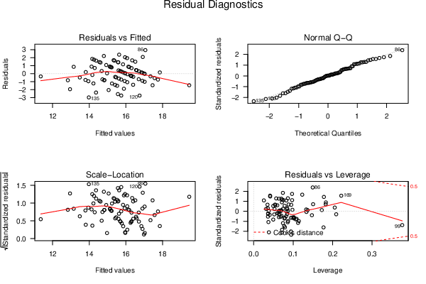
| Menu of Residual Diagnostics | |
| Description | Link |
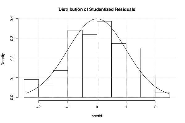
| Histogram | Compute |
| Central Tendency | Compute |
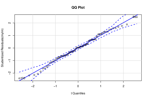
| QQ Plot | Compute |
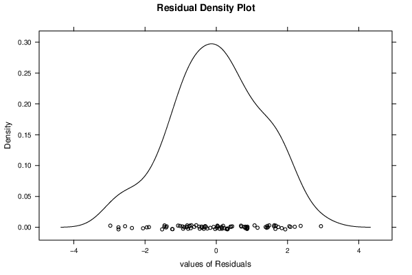
| Kernel Density Plot | Compute |
| Skewness/Kurtosis Test | Compute |
| Skewness-Kurtosis Plot | Compute |
| Harrell-Davis Plot | Compute |
| Bootstrap Plot -- Central Tendency | Compute |
| Blocked Bootstrap Plot -- Central Tendency | Compute |
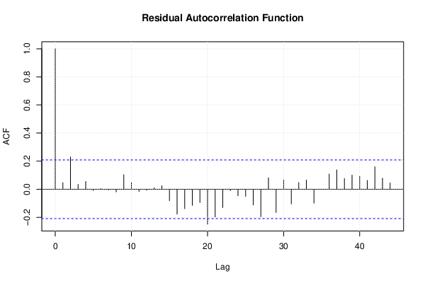
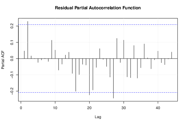
| (Partial) Autocorrelation Plot | Compute |
| Spectral Analysis | Compute |
| Tukey lambda PPCC Plot | Compute |
| Box-Cox Normality Plot | Compute |
| Summary Statistics | Compute |
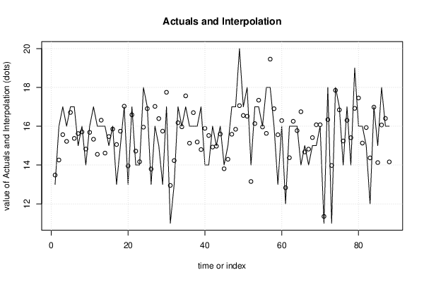
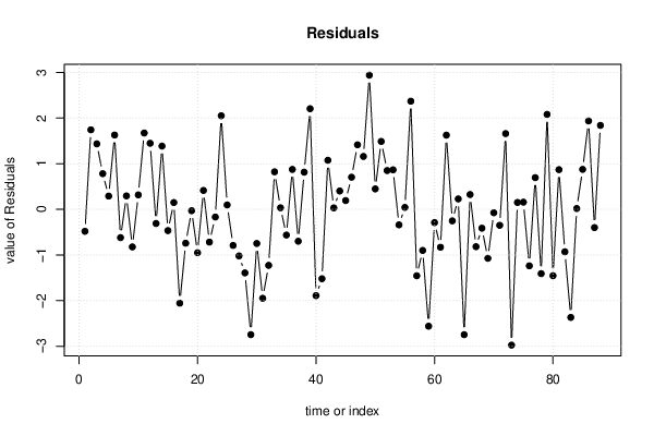
| Multiple Linear Regression - Actuals, Interpolation, and Residuals | |||
| Time or Index | Actuals | Interpolation Forecast | Residuals Prediction Error |
| 1 | 13 | 13.48 | -0.4826 |
| 2 | 16 | 14.26 | 1.741 |
| 3 | 17 | 15.57 | 1.434 |
| 4 | 16 | 15.22 | 0.7803 |
| 5 | 17 | 16.71 | 0.2898 |
| 6 | 17 | 15.37 | 1.627 |
| 7 | 15 | 15.62 | -0.6214 |
| 8 | 16 | 15.71 | 0.2935 |
| 9 | 14 | 14.82 | -0.8245 |
| 10 | 16 | 15.69 | 0.315 |
| 11 | 17 | 15.33 | 1.671 |
| 12 | 16 | 14.55 | 1.446 |
| 13 | 16 | 16.31 | -0.3109 |
| 14 | 16 | 14.62 | 1.385 |
| 15 | 15 | 15.47 | -0.4672 |
| 16 | 16 | 15.85 | 0.1479 |
| 17 | 13 | 15.06 | -2.057 |
| 18 | 15 | 15.74 | -0.7434 |
| 19 | 17 | 17.03 | -0.0311 |
| 20 | 13 | 13.95 | -0.9524 |
| 21 | 17 | 16.59 | 0.413 |
| 22 | 14 | 14.72 | -0.7184 |
| 23 | 14 | 14.17 | -0.1698 |
| 24 | 18 | 15.95 | 2.049 |
| 25 | 17 | 16.91 | 0.09427 |
| 26 | 13 | 13.79 | -0.7918 |
| 27 | 16 | 17.02 | -1.022 |
| 28 | 15 | 16.39 | -1.394 |
| 29 | 13 | 15.75 | -2.747 |
| 30 | 17 | 17.75 | -0.7493 |
| 31 | 11 | 12.95 | -1.95 |
| 32 | 13 | 14.23 | -1.228 |
| 33 | 17 | 16.18 | 0.8207 |
| 34 | 16 | 15.97 | 0.03216 |
| 35 | 17 | 17.56 | -0.5644 |
| 36 | 16 | 15.13 | 0.8734 |
| 37 | 16 | 16.7 | -0.6996 |
| 38 | 16 | 15.19 | 0.8133 |
| 39 | 17 | 14.8 | 2.203 |
| 40 | 14 | 15.89 | -1.891 |
| 41 | 14 | 15.52 | -1.522 |
| 42 | 16 | 14.93 | 1.074 |
| 43 | 15 | 14.97 | 0.03101 |
| 44 | 16 | 15.6 | 0.4011 |
| 45 | 14 | 13.81 | 0.1911 |
| 46 | 15 | 14.3 | 0.7026 |
| 47 | 17 | 15.59 | 1.413 |
| 48 | 17 | 15.84 | 1.158 |
| 49 | 20 | 17.06 | 2.939 |
| 50 | 17 | 16.55 | 0.4465 |
| 51 | 18 | 16.51 | 1.486 |
| 52 | 14 | 13.15 | 0.849 |
| 53 | 17 | 16.14 | 0.8646 |
| 54 | 17 | 17.34 | -0.3412 |
| 55 | 16 | 15.96 | 0.04096 |
| 56 | 18 | 15.63 | 2.368 |
| 57 | 18 | 19.46 | -1.456 |
| 58 | 16 | 16.9 | -0.9015 |
| 59 | 13 | 15.56 | -2.562 |
| 60 | 16 | 16.29 | -0.2915 |
| 61 | 12 | 12.83 | -0.8316 |
| 62 | 16 | 14.38 | 1.624 |
| 63 | 16 | 16.25 | -0.2535 |
| 64 | 16 | 15.77 | 0.2272 |
| 65 | 14 | 16.75 | -2.748 |
| 66 | 15 | 14.68 | 0.3232 |
| 67 | 14 | 14.82 | -0.8193 |
| 68 | 15 | 15.41 | -0.4141 |
| 69 | 15 | 16.07 | -1.074 |
| 70 | 16 | 16.08 | -0.07599 |
| 71 | 11 | 11.35 | -0.3516 |
| 72 | 18 | 16.34 | 1.658 |
| 73 | 11 | 13.98 | -2.977 |
| 74 | 18 | 17.85 | 0.1497 |
| 75 | 17 | 16.84 | 0.1559 |
| 76 | 14 | 15.24 | -1.239 |
| 77 | 17 | 16.31 | 0.6934 |
| 78 | 14 | 15.41 | -1.41 |
| 79 | 19 | 16.92 | 2.079 |
| 80 | 16 | 17.46 | -1.455 |
| 81 | 16 | 15.13 | 0.8686 |
| 82 | 15 | 15.93 | -0.9314 |
| 83 | 12 | 14.37 | -2.369 |
| 84 | 17 | 16.98 | 0.0169 |
| 85 | 15 | 14.13 | 0.8745 |
| 86 | 18 | 16.06 | 1.936 |
| 87 | 16 | 16.4 | -0.4012 |
| 88 | 16 | 14.16 | 1.838 |
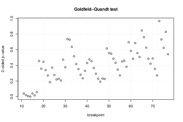
| Goldfeld-Quandt test for Heteroskedasticity | |||
| p-values | Alternative Hypothesis | ||
| breakpoint index | greater | 2-sided | less |
| 11 | 0.02055 | 0.0411 | 0.9795 |
| 12 | 0.01012 | 0.02025 | 0.9899 |
| 13 | 0.003408 | 0.006815 | 0.9966 |
| 14 | 0.0009154 | 0.001831 | 0.9991 |
| 15 | 0.02102 | 0.04204 | 0.979 |
| 16 | 0.008694 | 0.01739 | 0.9913 |
| 17 | 0.02951 | 0.05902 | 0.9705 |
| 18 | 0.2283 | 0.4566 | 0.7717 |
| 19 | 0.1789 | 0.3578 | 0.8211 |
| 20 | 0.2233 | 0.4466 | 0.7767 |
| 21 | 0.1705 | 0.3409 | 0.8295 |
| 22 | 0.1354 | 0.2709 | 0.8646 |
| 23 | 0.09326 | 0.1865 | 0.9067 |
| 24 | 0.1858 | 0.3716 | 0.8142 |
| 25 | 0.1383 | 0.2765 | 0.8617 |
| 26 | 0.1103 | 0.2206 | 0.8897 |
| 27 | 0.1146 | 0.2292 | 0.8854 |
| 28 | 0.1036 | 0.2073 | 0.8964 |
| 29 | 0.237 | 0.474 | 0.763 |
| 30 | 0.1887 | 0.3773 | 0.8113 |
| 31 | 0.3684 | 0.7368 | 0.6316 |
| 32 | 0.3642 | 0.7285 | 0.6358 |
| 33 | 0.3187 | 0.6374 | 0.6813 |
| 34 | 0.2584 | 0.5169 | 0.7416 |
| 35 | 0.2088 | 0.4176 | 0.7912 |
| 36 | 0.1766 | 0.3532 | 0.8234 |
| 37 | 0.1404 | 0.2807 | 0.8596 |
| 38 | 0.1177 | 0.2354 | 0.8823 |
| 39 | 0.1651 | 0.3301 | 0.8349 |
| 40 | 0.2155 | 0.431 | 0.7845 |
| 41 | 0.2388 | 0.4776 | 0.7612 |
| 42 | 0.227 | 0.4539 | 0.773 |
| 43 | 0.1839 | 0.3677 | 0.8161 |
| 44 | 0.1468 | 0.2936 | 0.8532 |
| 45 | 0.1148 | 0.2295 | 0.8852 |
| 46 | 0.09616 | 0.1923 | 0.9038 |
| 47 | 0.116 | 0.232 | 0.884 |
| 48 | 0.1137 | 0.2275 | 0.8863 |
| 49 | 0.3083 | 0.6166 | 0.6917 |
| 50 | 0.2785 | 0.5571 | 0.7215 |
| 51 | 0.2751 | 0.5501 | 0.7249 |
| 52 | 0.243 | 0.4861 | 0.757 |
| 53 | 0.2162 | 0.4323 | 0.7838 |
| 54 | 0.1733 | 0.3465 | 0.8267 |
| 55 | 0.1359 | 0.2718 | 0.8641 |
| 56 | 0.2245 | 0.4491 | 0.7755 |
| 57 | 0.2302 | 0.4604 | 0.7698 |
| 58 | 0.1917 | 0.3834 | 0.8083 |
| 59 | 0.3479 | 0.6958 | 0.6521 |
| 60 | 0.292 | 0.584 | 0.708 |
| 61 | 0.2424 | 0.4848 | 0.7576 |
| 62 | 0.3431 | 0.6861 | 0.6569 |
| 63 | 0.2786 | 0.5572 | 0.7214 |
| 64 | 0.2537 | 0.5075 | 0.7463 |
| 65 | 0.4234 | 0.8468 | 0.5766 |
| 66 | 0.3802 | 0.7605 | 0.6198 |
| 67 | 0.3137 | 0.6274 | 0.6863 |
| 68 | 0.243 | 0.4859 | 0.757 |
| 69 | 0.2113 | 0.4227 | 0.7887 |
| 70 | 0.2447 | 0.4894 | 0.7553 |
| 71 | 0.1778 | 0.3557 | 0.8222 |
| 72 | 0.1362 | 0.2723 | 0.8638 |
| 73 | 0.4835 | 0.9669 | 0.5165 |
| 74 | 0.3659 | 0.7318 | 0.6341 |
| 75 | 0.3121 | 0.6241 | 0.6879 |
| 76 | 0.4142 | 0.8285 | 0.5858 |
| 77 | 0.2713 | 0.5425 | 0.7287 |
| Meta Analysis of Goldfeld-Quandt test for Heteroskedasticity | |||
| Description | # significant tests | % significant tests | OK/NOK |
| 1% type I error level | 2 | 0.02985 | NOK |
| 5% type I error level | 6 | 0.0895522 | NOK |
| 10% type I error level | 7 | 0.104478 | NOK |
| Ramsey RESET F-Test for powers (2 and 3) of fitted values |
> reset_test_fitted RESET test data: mylm RESET = 1.651, df1 = 2, df2 = 78, p-value = 0.1985 |
| Ramsey RESET F-Test for powers (2 and 3) of regressors |
> reset_test_regressors RESET test data: mylm RESET = 1.1562, df1 = 14, df2 = 66, p-value = 0.3292 |
| Ramsey RESET F-Test for powers (2 and 3) of principal components |
> reset_test_principal_components RESET test data: mylm RESET = 1.5993, df1 = 2, df2 = 78, p-value = 0.2086 |
| Variance Inflation Factors (Multicollinearity) |
> vif `SK/EOU1` `SK/EOU2` `SK/EOU4` IKSUM GW1 GW2 ECSUM 1.138869 1.230208 1.092730 1.050695 1.083880 1.067510 1.023205 |