Free Statistics
of Irreproducible Research!
Description of Statistical Computation | ||||||||||||||||||||||||||||||||||||||||||||||||
|---|---|---|---|---|---|---|---|---|---|---|---|---|---|---|---|---|---|---|---|---|---|---|---|---|---|---|---|---|---|---|---|---|---|---|---|---|---|---|---|---|---|---|---|---|---|---|---|---|
| Author's title | ||||||||||||||||||||||||||||||||||||||||||||||||
| Author | *The author of this computation has been verified* | |||||||||||||||||||||||||||||||||||||||||||||||
| R Software Module | rwasp_fitdistrnorm.wasp | |||||||||||||||||||||||||||||||||||||||||||||||
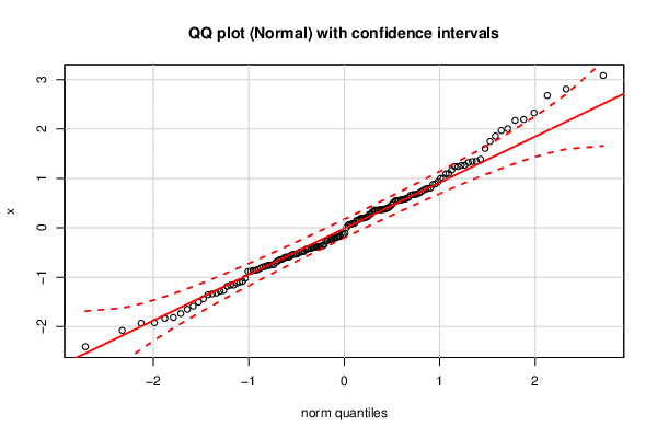
| Title produced by software | ML Fitting and QQ Plot- Normal Distribution | |||||||||||||||||||||||||||||||||||||||||||||||
| Date of computation | Tue, 09 Oct 2018 14:09:47 +0200 | |||||||||||||||||||||||||||||||||||||||||||||||
| Cite this page as follows | Statistical Computations at FreeStatistics.org, Office for Research Development and Education, URL https://freestatistics.org/blog/index.php?v=date/2018/Oct/09/t1539087049zhtx85xtbhrug6c.htm/, Retrieved Tue, 07 May 2024 13:29:11 +0000 | |||||||||||||||||||||||||||||||||||||||||||||||
| Statistical Computations at FreeStatistics.org, Office for Research Development and Education, URL https://freestatistics.org/blog/index.php?pk=315573, Retrieved Tue, 07 May 2024 13:29:11 +0000 | ||||||||||||||||||||||||||||||||||||||||||||||||
| QR Codes: | ||||||||||||||||||||||||||||||||||||||||||||||||
|
| ||||||||||||||||||||||||||||||||||||||||||||||||
| Original text written by user: | ||||||||||||||||||||||||||||||||||||||||||||||||
| IsPrivate? | No (this computation is public) | |||||||||||||||||||||||||||||||||||||||||||||||
| User-defined keywords | ||||||||||||||||||||||||||||||||||||||||||||||||
| Estimated Impact | 130 | |||||||||||||||||||||||||||||||||||||||||||||||
Tree of Dependent Computations | ||||||||||||||||||||||||||||||||||||||||||||||||
| Family? (F = Feedback message, R = changed R code, M = changed R Module, P = changed Parameters, D = changed Data) | ||||||||||||||||||||||||||||||||||||||||||||||||
| - [ML Fitting and QQ Plot- Normal Distribution] [H3 Task 3] [2018-10-09 12:09:47] [9e2b27cf675a1d7b8e7da04c0e26bb6a] [Current] | ||||||||||||||||||||||||||||||||||||||||||||||||
| Feedback Forum | ||||||||||||||||||||||||||||||||||||||||||||||||
Post a new message | ||||||||||||||||||||||||||||||||||||||||||||||||
Dataset | ||||||||||||||||||||||||||||||||||||||||||||||||
| Dataseries X: | ||||||||||||||||||||||||||||||||||||||||||||||||
-0.862918028 -0.5357396682 0.7025423657 0.7967613424 0.4005979966 -0.1297588914 -0.6693075465 0.8773356872 1.268363075 -1.118383686 -0.747627293 0.1765713862 0.1569479667 0.8875086715 -0.48524868 -0.4179981081 1.85620947 -0.345491976 -0.1691755425 -0.7492213275 0.3760925247 -1.502308018 0.1996550111 0.8041291287 -1.159693123 0.9985211341 0.5734874439 -1.931310049 0.4268787105 0.2696100203 -0.4282637037 0.3647147286 0.355577453 -0.2336277557 -0.7581485635 1.341157069 -2.077782297 -1.354459039 -0.1329436843 0.3576288507 0.579835713 0.6705647622 -0.1790370314 -0.5867672006 0.06674139608 -1.336122202 -0.5309392059 -0.3777290965 -0.41855507 0.506045426 -0.8829187695 -0.763172828 2.004458558 0.6817848726 1.006236599 -0.7837742269 1.166973303 0.3728605134 -0.6446654698 1.343363823 -1.833589113 1.097854418 -0.5502326996 -0.1120801276 0.7288501977 -1.101188053 -0.2226237522 -1.183563706 0.6183294507 0.07476223971 0.2111904273 0.5492776818 0.09302249218 0.4621136667 1.23904146 -1.735536126 -0.5917089436 1.261924335 1.240052596 1.748377769 0.366610877 -1.585952204 2.808002969 -0.2066515316 -1.085625784 -0.481846802 -0.8784332616 -0.8578907768 0.7855658132 -0.6983788532 -0.6385724452 -1.020869618 0.192315392 -0.3656861704 2.174267705 1.968827635 0.5623239076 0.09022098435 -0.8163676699 -1.159355312 0.3231656228 0.05598004213 0.5476688087 -0.4789883251 -1.266535474 -0.6137282586 -1.436259124 -0.1878223366 -0.2390535755 1.606090796 1.319918009 -0.3820808209 0.007365513421 0.6598911389 0.3933395802 -1.283877282 -1.31969381 -0.792393599 0.5954541121 -1.921756717 -0.3881402836 -0.532453948 0.7641337292 -0.2643630967 2.324176154 -0.3938350424 -0.3973368494 2.192768935 0.1418911216 0.6747095993 -0.434395945 1.387297058 -1.648572702 1.092738215 -0.2084655812 0.1970289883 -0.592828621 2.678516502 3.082662706 -0.5062440029 -1.815474193 0.2262880424 0.9313170451 -0.2560395684 0.2798356406 -0.3695801694 -2.406690353 -0.843601073 0.3571899308 0.556422793 | ||||||||||||||||||||||||||||||||||||||||||||||||
Tables (Output of Computation) | ||||||||||||||||||||||||||||||||||||||||||||||||
| ||||||||||||||||||||||||||||||||||||||||||||||||
Figures (Output of Computation) | ||||||||||||||||||||||||||||||||||||||||||||||||
Input Parameters & R Code | ||||||||||||||||||||||||||||||||||||||||||||||||
| Parameters (Session): | ||||||||||||||||||||||||||||||||||||||||||||||||
| par1 = 8 ; par2 = 0 ; | ||||||||||||||||||||||||||||||||||||||||||||||||
| Parameters (R input): | ||||||||||||||||||||||||||||||||||||||||||||||||
| par1 = 8 ; par2 = 0 ; | ||||||||||||||||||||||||||||||||||||||||||||||||
| R code (references can be found in the software module): | ||||||||||||||||||||||||||||||||||||||||||||||||
par2 <- '0' | ||||||||||||||||||||||||||||||||||||||||||||||||