Free Statistics
of Irreproducible Research!
Description of Statistical Computation | ||||||||||||||||||||||||||||||||||||||||||||||||
|---|---|---|---|---|---|---|---|---|---|---|---|---|---|---|---|---|---|---|---|---|---|---|---|---|---|---|---|---|---|---|---|---|---|---|---|---|---|---|---|---|---|---|---|---|---|---|---|---|
| Author's title | ||||||||||||||||||||||||||||||||||||||||||||||||
| Author | *The author of this computation has been verified* | |||||||||||||||||||||||||||||||||||||||||||||||
| R Software Module | rwasp_fitdistrnorm.wasp | |||||||||||||||||||||||||||||||||||||||||||||||
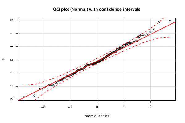
| Title produced by software | ML Fitting and QQ Plot- Normal Distribution | |||||||||||||||||||||||||||||||||||||||||||||||
| Date of computation | Thu, 04 Oct 2018 13:06:24 +0200 | |||||||||||||||||||||||||||||||||||||||||||||||
| Cite this page as follows | Statistical Computations at FreeStatistics.org, Office for Research Development and Education, URL https://freestatistics.org/blog/index.php?v=date/2018/Oct/04/t1538651204gc2mbcwd5dtl6f2.htm/, Retrieved Fri, 03 May 2024 15:23:38 +0000 | |||||||||||||||||||||||||||||||||||||||||||||||
| Statistical Computations at FreeStatistics.org, Office for Research Development and Education, URL https://freestatistics.org/blog/index.php?pk=315556, Retrieved Fri, 03 May 2024 15:23:38 +0000 | ||||||||||||||||||||||||||||||||||||||||||||||||
| QR Codes: | ||||||||||||||||||||||||||||||||||||||||||||||||
|
| ||||||||||||||||||||||||||||||||||||||||||||||||
| Original text written by user: | ||||||||||||||||||||||||||||||||||||||||||||||||
| IsPrivate? | No (this computation is public) | |||||||||||||||||||||||||||||||||||||||||||||||
| User-defined keywords | ||||||||||||||||||||||||||||||||||||||||||||||||
| Estimated Impact | 95 | |||||||||||||||||||||||||||||||||||||||||||||||
Tree of Dependent Computations | ||||||||||||||||||||||||||||||||||||||||||||||||
| Family? (F = Feedback message, R = changed R code, M = changed R Module, P = changed Parameters, D = changed Data) | ||||||||||||||||||||||||||||||||||||||||||||||||
| - [ML Fitting and QQ Plot- Normal Distribution] [] [2018-10-04 11:06:24] [679f1112dc3b31869254dd82340bfb0d] [Current] | ||||||||||||||||||||||||||||||||||||||||||||||||
| Feedback Forum | ||||||||||||||||||||||||||||||||||||||||||||||||
Post a new message | ||||||||||||||||||||||||||||||||||||||||||||||||
Dataset | ||||||||||||||||||||||||||||||||||||||||||||||||
| Dataseries X: | ||||||||||||||||||||||||||||||||||||||||||||||||
1.387349497 -0.7014523818 -0.7989135642 -0.9624411739 -1.699873857 2.879561752 0.02589333558 0.6019187574 -1.13053661 -0.2681588565 -0.3354257686 -0.4999781263 -1.20983967 -0.3446480965 -1.164467106 1.093845484 -2.818668577 -0.7451005762 -1.050627925 -0.7619885569 0.7745170479 0.5930823026 -2.148309012 -0.2625726808 -0.288831435 -0.04737861336 0.1752584301 1.914303333 -0.05049105512 -0.2919360085 -0.6984397127 -0.7154563262 1.280768039 -0.6931369691 -0.06827704386 -0.6564865222 -0.0452071716 -0.6401689294 1.266810458 -0.5388200649 0.9150329637 -0.1590306786 0.7974979473 1.886629462 -0.3570990786 1.39667187 -0.2968807 0.8619586208 -1.388492415 1.764304891 -0.139910289 -1.15445857 0.3487722074 2.300160359 -1.540295929 -0.1553295873 1.109908196 -0.3832143757 -0.7646906794 0.8575735608 0.1592831794 0.3296871255 0.2988526193 0.4248056377 -0.3383454055 -1.086590272 -0.4131958124 0.2900152116 -0.8172202489 -0.3330091544 -0.08454513868 0.1700855553 -0.2005986257 -0.2112108162 -0.3544106043 -0.3653478764 -0.1813919639 0.5606894245 -0.04346620747 0.09499345094 0.1065692204 -0.3583192106 1.729578722 0.9022980005 0.02664584145 -1.529188607 0.0407768599 0.5553058342 0.9868757981 -1.220482585 1.263116103 -0.9826748083 -0.403166136 -0.7866730107 -0.2219327864 1.14262392 -0.5661325366 1.062939464 1.296506749 0.2121964497 -1.581293233 -1.895320535 -1.210985116 0.5789048989 -1.199549712 -1.449674096 -0.9744517202 1.421995971 0.7509248539 -1.893683667 -0.2755119197 -1.389007352 -0.4315786784 -0.8576743153 1.311062465 -1.321039399 -1.509195214 1.969220715 -1.714855472 0.9051497877 -1.882000203 1.226388797 0.1984256295 0.5070111595 0.4438511511 0.3784423664 0.2409626343 -2.058411713 0.4973585693 1.321297663 -0.562899099 -2.683716234 -0.406712293 -0.9023707791 0.4507724724 -1.090998996 1.192155055 0.7216984309 0.0001686464565 -2.202339197 0.3695885442 2.113558249 0.8817876717 0.5990928802 1.895062789 -1.857367946 0.603858031 -0.6826974852 2.920009433 -0.2193326272 | ||||||||||||||||||||||||||||||||||||||||||||||||
Tables (Output of Computation) | ||||||||||||||||||||||||||||||||||||||||||||||||
| ||||||||||||||||||||||||||||||||||||||||||||||||
Figures (Output of Computation) | ||||||||||||||||||||||||||||||||||||||||||||||||
Input Parameters & R Code | ||||||||||||||||||||||||||||||||||||||||||||||||
| Parameters (Session): | ||||||||||||||||||||||||||||||||||||||||||||||||
| par1 = 8 ; par2 = 0 ; | ||||||||||||||||||||||||||||||||||||||||||||||||
| Parameters (R input): | ||||||||||||||||||||||||||||||||||||||||||||||||
| par1 = 8 ; par2 = 0 ; | ||||||||||||||||||||||||||||||||||||||||||||||||
| R code (references can be found in the software module): | ||||||||||||||||||||||||||||||||||||||||||||||||
library(MASS) | ||||||||||||||||||||||||||||||||||||||||||||||||