| Multiple Linear Regression - Estimated Regression Equation |
| GWSUM[t] = + 14.7832 + 0.138622IK1[t] + 0.153261IK2[t] -0.485353IK3[t] + 0.0132018IK4[t] + 0.000686423KVDD1[t] + 0.225461KVDD2[t] -0.0870457KVDD3[t] -0.0388076KVDD4[t] -0.24919`SK/EOU1`[t] + 0.548165`SK/EOU2`[t] -0.0398974`SK/EOU3`[t] -0.15473`SK/EOU4`[t] -0.252386`SK/EOU5`[t] -0.400778`SK/EOU6`[t] + e[t] |
| Multiple Linear Regression - Ordinary Least Squares | |||||
| Variable | Parameter | S.D. | T-STAT H0: parameter = 0 | 2-tail p-value | 1-tail p-value |
| (Intercept) | +14.78 | 3.102 | +4.7650e+00 | 9.903e-06 | 4.952e-06 |
| IK1 | +0.1386 | 0.3432 | +4.0380e-01 | 0.6876 | 0.3438 |
| IK2 | +0.1533 | 0.2778 | +5.5160e-01 | 0.583 | 0.2915 |
| IK3 | -0.4854 | 0.3445 | -1.4090e+00 | 0.1633 | 0.08163 |
| IK4 | +0.0132 | 0.2966 | +4.4510e-02 | 0.9646 | 0.4823 |
| KVDD1 | +0.0006864 | 0.2334 | +2.9410e-03 | 0.9977 | 0.4988 |
| KVDD2 | +0.2255 | 0.1722 | +1.3090e+00 | 0.1947 | 0.09734 |
| KVDD3 | -0.08705 | 0.2004 | -4.3440e-01 | 0.6653 | 0.3327 |
| KVDD4 | -0.03881 | 0.2044 | -1.8980e-01 | 0.85 | 0.425 |
| `SK/EOU1` | -0.2492 | 0.2506 | -9.9440e-01 | 0.3234 | 0.1617 |
| `SK/EOU2` | +0.5482 | 0.2785 | +1.9680e+00 | 0.05301 | 0.02651 |
| `SK/EOU3` | -0.0399 | 0.2429 | -1.6420e-01 | 0.87 | 0.435 |
| `SK/EOU4` | -0.1547 | 0.3327 | -4.6510e-01 | 0.6433 | 0.3217 |
| `SK/EOU5` | -0.2524 | 0.2816 | -8.9630e-01 | 0.3731 | 0.1866 |
| `SK/EOU6` | -0.4008 | 0.2875 | -1.3940e+00 | 0.1678 | 0.08389 |
| Multiple Linear Regression - Regression Statistics | |
| Multiple R | 0.3617 |
| R-squared | 0.1308 |
| Adjusted R-squared | -0.04304 |
| F-TEST (value) | 0.7524 |
| F-TEST (DF numerator) | 14 |
| F-TEST (DF denominator) | 70 |
| p-value | 0.7149 |
| Multiple Linear Regression - Residual Statistics | |
| Residual Standard Deviation | 1.513 |
| Sum Squared Residuals | 160.2 |
| Menu of Residual Diagnostics | |
| Description | Link |
| Histogram | Compute |
| Central Tendency | Compute |
| QQ Plot | Compute |
| Kernel Density Plot | Compute |
| Skewness/Kurtosis Test | Compute |
| Skewness-Kurtosis Plot | Compute |
| Harrell-Davis Plot | Compute |
| Bootstrap Plot -- Central Tendency | Compute |
| Blocked Bootstrap Plot -- Central Tendency | Compute |
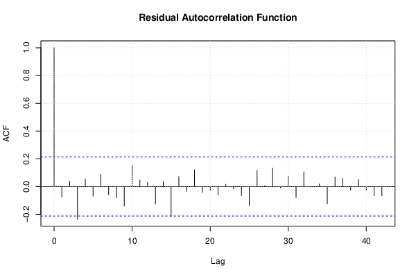
| (Partial) Autocorrelation Plot | Compute |
| Spectral Analysis | Compute |
| Tukey lambda PPCC Plot | Compute |
| Box-Cox Normality Plot | Compute |
| Summary Statistics | Compute |
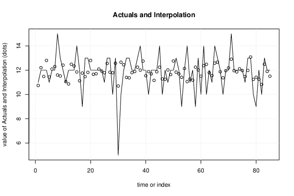
| Multiple Linear Regression - Actuals, Interpolation, and Residuals | |||
| Time or Index | Actuals | Interpolation Forecast | Residuals Prediction Error |
| 1 | 11 | 10.74 | 0.2574 |
| 2 | 12 | 12.21 | -0.2068 |
| 3 | 12 | 11.48 | 0.5154 |
| 4 | 12 | 12.8 | -0.8044 |
| 5 | 11 | 11.44 | -0.4412 |
| 6 | 12 | 12.09 | -0.0936 |
| 7 | 12 | 12.3 | -0.2972 |
| 8 | 15 | 11.6 | 3.397 |
| 9 | 13 | 11.52 | 1.478 |
| 10 | 12 | 12.42 | -0.4191 |
| 11 | 11 | 11.05 | -0.05408 |
| 12 | 12 | 10.87 | 1.134 |
| 13 | 12 | 12.49 | -0.4892 |
| 14 | 12 | 12.34 | -0.3418 |
| 15 | 14 | 11.85 | 2.146 |
| 16 | 12 | 11.13 | 0.871 |
| 17 | 9 | 11.76 | -2.763 |
| 18 | 13 | 11.47 | 1.528 |
| 19 | 13 | 11.82 | 1.18 |
| 20 | 12 | 12.8 | -0.8034 |
| 21 | 12 | 11.66 | 0.3398 |
| 22 | 12 | 11.71 | 0.293 |
| 23 | 12 | 12.09 | -0.09445 |
| 24 | 12 | 11.93 | 0.06669 |
| 25 | 11 | 11.79 | -0.7907 |
| 26 | 13 | 12.56 | 0.4403 |
| 27 | 13 | 11.84 | 1.164 |
| 28 | 10 | 11.79 | -1.791 |
| 29 | 13 | 12.57 | 0.4298 |
| 30 | 5 | 10.7 | -5.696 |
| 31 | 10 | 12.66 | -2.655 |
| 32 | 12 | 12.45 | -0.4464 |
| 33 | 13 | 11.41 | 1.595 |
| 34 | 13 | 11.37 | 1.63 |
| 35 | 12 | 11.8 | 0.2002 |
| 36 | 12 | 11.89 | 0.1128 |
| 37 | 13 | 12.25 | 0.7505 |
| 38 | 14 | 12.01 | 1.994 |
| 39 | 12 | 12.75 | -0.7487 |
| 40 | 12 | 11.55 | 0.4547 |
| 41 | 10 | 11.89 | -1.886 |
| 42 | 12 | 11.7 | 0.3006 |
| 43 | 12 | 11.16 | 0.8386 |
| 44 | 12 | 11.87 | 0.1322 |
| 45 | 14 | 12.25 | 1.754 |
| 46 | 10 | 11.28 | -1.278 |
| 47 | 12 | 11.26 | 0.7438 |
| 48 | 11 | 12.02 | -1.025 |
| 49 | 12 | 11.64 | 0.3593 |
| 50 | 12 | 12.76 | -0.7583 |
| 51 | 13 | 11.84 | 1.161 |
| 52 | 12 | 11.69 | 0.3054 |
| 53 | 9 | 11.41 | -2.413 |
| 54 | 12 | 12.14 | -0.1356 |
| 55 | 14 | 11.06 | 2.942 |
| 56 | 11 | 11.27 | -0.267 |
| 57 | 12 | 11.18 | 0.8204 |
| 58 | 9 | 12.25 | -3.253 |
| 59 | 13 | 12.02 | 0.9766 |
| 60 | 10 | 11.51 | -1.507 |
| 61 | 14 | 12.37 | 1.628 |
| 62 | 10 | 12.48 | -2.485 |
| 63 | 12 | 11.8 | 0.2008 |
| 64 | 11 | 11.56 | -0.5586 |
| 65 | 14 | 12.58 | 1.416 |
| 66 | 13 | 12.66 | 0.3363 |
| 67 | 12 | 11.87 | 0.1321 |
| 68 | 10 | 11.37 | -1.372 |
| 69 | 12 | 11.96 | 0.03936 |
| 70 | 12 | 12.19 | -0.1927 |
| 71 | 15 | 12.91 | 2.093 |
| 72 | 12 | 11.96 | 0.03805 |
| 73 | 12 | 11.86 | 0.1405 |
| 74 | 12 | 12.11 | -0.109 |
| 75 | 12 | 11.97 | 0.03113 |
| 76 | 11 | 11.48 | -0.4798 |
| 77 | 13 | 11.98 | 1.017 |
| 78 | 13 | 13.08 | -0.08381 |
| 79 | 10 | 11.24 | -1.245 |
| 80 | 9 | 11.42 | -2.421 |
| 81 | 12 | 11.26 | 0.7431 |
| 82 | 10 | 10.82 | -0.8242 |
| 83 | 13 | 12.5 | 0.5032 |
| 84 | 12 | 11.9 | 0.1047 |
| 85 | 12 | 11.5 | 0.4952 |
| Goldfeld-Quandt test for Heteroskedasticity | |||
| p-values | Alternative Hypothesis | ||
| breakpoint index | greater | 2-sided | less |
| 18 | 0.6436 | 0.7128 | 0.3564 |
| 19 | 0.533 | 0.934 | 0.467 |
| 20 | 0.6444 | 0.7113 | 0.3556 |
| 21 | 0.5836 | 0.8327 | 0.4164 |
| 22 | 0.4605 | 0.9209 | 0.5395 |
| 23 | 0.3569 | 0.7139 | 0.6431 |
| 24 | 0.2861 | 0.5722 | 0.7139 |
| 25 | 0.2138 | 0.4276 | 0.7862 |
| 26 | 0.2068 | 0.4136 | 0.7932 |
| 27 | 0.2541 | 0.5082 | 0.7459 |
| 28 | 0.2454 | 0.4909 | 0.7546 |
| 29 | 0.1893 | 0.3785 | 0.8107 |
| 30 | 0.9526 | 0.09489 | 0.04745 |
| 31 | 0.9708 | 0.05842 | 0.02921 |
| 32 | 0.963 | 0.074 | 0.037 |
| 33 | 0.9567 | 0.08651 | 0.04326 |
| 34 | 0.9543 | 0.09136 | 0.04568 |
| 35 | 0.9322 | 0.1356 | 0.06781 |
| 36 | 0.9073 | 0.1854 | 0.09268 |
| 37 | 0.8753 | 0.2494 | 0.1247 |
| 38 | 0.8856 | 0.2288 | 0.1144 |
| 39 | 0.8504 | 0.2993 | 0.1496 |
| 40 | 0.8119 | 0.3762 | 0.1881 |
| 41 | 0.8424 | 0.3153 | 0.1576 |
| 42 | 0.7926 | 0.4148 | 0.2074 |
| 43 | 0.7506 | 0.4988 | 0.2494 |
| 44 | 0.6899 | 0.6202 | 0.3101 |
| 45 | 0.7168 | 0.5663 | 0.2832 |
| 46 | 0.7144 | 0.5711 | 0.2856 |
| 47 | 0.669 | 0.662 | 0.331 |
| 48 | 0.7764 | 0.4472 | 0.2236 |
| 49 | 0.724 | 0.5521 | 0.276 |
| 50 | 0.6551 | 0.6898 | 0.3449 |
| 51 | 0.6916 | 0.6168 | 0.3084 |
| 52 | 0.627 | 0.7459 | 0.373 |
| 53 | 0.8423 | 0.3154 | 0.1577 |
| 54 | 0.8159 | 0.3681 | 0.184 |
| 55 | 0.9351 | 0.1297 | 0.06485 |
| 56 | 0.9175 | 0.1651 | 0.08254 |
| 57 | 0.9683 | 0.06331 | 0.03165 |
| 58 | 0.9968 | 0.00637 | 0.003185 |
| 59 | 0.9931 | 0.01387 | 0.006934 |
| 60 | 0.9874 | 0.02528 | 0.01264 |
| 61 | 0.9833 | 0.03349 | 0.01675 |
| 62 | 0.9921 | 0.0158 | 0.007898 |
| 63 | 0.9999 | 0.0001463 | 7.317e-05 |
| 64 | 0.9996 | 0.0007894 | 0.0003947 |
| 65 | 0.9982 | 0.003617 | 0.001808 |
| 66 | 0.9948 | 0.01039 | 0.005197 |
| 67 | 0.9765 | 0.04692 | 0.02346 |
| Meta Analysis of Goldfeld-Quandt test for Heteroskedasticity | |||
| Description | # significant tests | % significant tests | OK/NOK |
| 1% type I error level | 4 | 0.08 | NOK |
| 5% type I error level | 10 | 0.2 | NOK |
| 10% type I error level | 16 | 0.32 | NOK |
| Ramsey RESET F-Test for powers (2 and 3) of fitted values |
> reset_test_fitted RESET test data: mylm RESET = 2.7706, df1 = 2, df2 = 68, p-value = 0.0697 |
| Ramsey RESET F-Test for powers (2 and 3) of regressors |
> reset_test_regressors RESET test data: mylm RESET = 0.8361, df1 = 28, df2 = 42, p-value = 0.6874 |
| Ramsey RESET F-Test for powers (2 and 3) of principal components |
> reset_test_principal_components RESET test data: mylm RESET = 0.10566, df1 = 2, df2 = 68, p-value = 0.8999 |
| Variance Inflation Factors (Multicollinearity) |
> vif
      IK1       IK2       IK3       IK4     KVDD1     KVDD2     KVDD3     KVDD4
 1.542067  1.319036  1.705432  1.290774  1.168808  1.128414  1.220570  1.261831
`SK/EOU1` `SK/EOU2` `SK/EOU3` `SK/EOU4` `SK/EOU5` `SK/EOU6`
 1.360240  1.302373  1.145574  1.175605  1.143655  1.116096
|