| Multiple Linear Regression - Estimated Regression Equation |
| barrels_purchased[t] = -6894.98 -644.366unit_price[t] + 109889defl_price1[t] + 24133.2dum[t] + 597.488US_IND_PROD[t] -145145defl_price1dum[t] + 0.256361`barrels_purchased(t-1)`[t] + 0.248871`barrels_purchased(t-2)`[t] + 0.182822`barrels_purchased(t-3)`[t] + 0.208868`barrels_purchased(t-1s)`[t] + 3815.37M1[t] -186.403M2[t] -661.025M3[t] -714.16M4[t] -12688.4M5[t] -8040.19M6[t] -14738.3M7[t] -11691.4M8[t] -3075.78M9[t] -24301.5M10[t] -4841.88M11[t] -27.0577t + e[t] |
| Warning: you did not specify the column number of the endogenous series! The first column was selected by default. |
| Multiple Linear Regression - Ordinary Least Squares | |||||
| Variable | Parameter | S.D. | T-STAT H0: parameter = 0 | 2-tail p-value | 1-tail p-value |
| (Intercept) | -6895 | 1.104e+04 | -6.2450e-01 | 0.5326 | 0.2663 |
| unit_price | -644.4 | 397.2 | -1.6220e+00 | 0.1055 | 0.05277 |
| defl_price1 | +1.099e+05 | 7.703e+04 | +1.4270e+00 | 0.1545 | 0.07726 |
| dum | +2.413e+04 | 9150 | +2.6370e+00 | 0.008695 | 0.004348 |
| US_IND_PROD | +597.5 | 299.9 | +1.9920e+00 | 0.04703 | 0.02351 |
| defl_price1dum | -1.451e+05 | 4.531e+04 | -3.2040e+00 | 0.001471 | 0.0007354 |
| `barrels_purchased(t-1)` | +0.2564 | 0.04954 | +5.1750e+00 | 3.692e-07 | 1.846e-07 |
| `barrels_purchased(t-2)` | +0.2489 | 0.04876 | +5.1040e+00 | 5.246e-07 | 2.623e-07 |
| `barrels_purchased(t-3)` | +0.1828 | 0.04852 | +3.7680e+00 | 0.0001907 | 9.536e-05 |
| `barrels_purchased(t-1s)` | +0.2089 | 0.04098 | +5.0970e+00 | 5.431e-07 | 2.716e-07 |
| M1 | +3815 | 4390 | +8.6900e-01 | 0.3854 | 0.1927 |
| M2 | -186.4 | 4213 | -4.4240e-02 | 0.9647 | 0.4824 |
| M3 | -661 | 4218 | -1.5670e-01 | 0.8755 | 0.4378 |
| M4 | -714.2 | 4200 | -1.7000e-01 | 0.8651 | 0.4325 |
| M5 | -1.269e+04 | 4249 | -2.9860e+00 | 0.003004 | 0.001502 |
| M6 | -8040 | 4272 | -1.8820e+00 | 0.06061 | 0.03031 |
| M7 | -1.474e+04 | 4130 | -3.5690e+00 | 0.0004044 | 0.0002022 |
| M8 | -1.169e+04 | 4262 | -2.7430e+00 | 0.006378 | 0.003189 |
| M9 | -3076 | 4110 | -7.4830e-01 | 0.4547 | 0.2274 |
| M10 | -2.43e+04 | 4310 | -5.6380e+00 | 3.354e-08 | 1.677e-08 |
| M11 | -4842 | 4436 | -1.0920e+00 | 0.2757 | 0.1378 |
| t | -27.06 | 58.88 | -4.5950e-01 | 0.6461 | 0.3231 |
| Multiple Linear Regression - Regression Statistics | |
| Multiple R | 0.9739 |
| R-squared | 0.9484 |
| Adjusted R-squared | 0.9455 |
| F-TEST (value) | 334.2 |
| F-TEST (DF numerator) | 21 |
| F-TEST (DF denominator) | 382 |
| p-value | 0 |
| Multiple Linear Regression - Residual Statistics | |
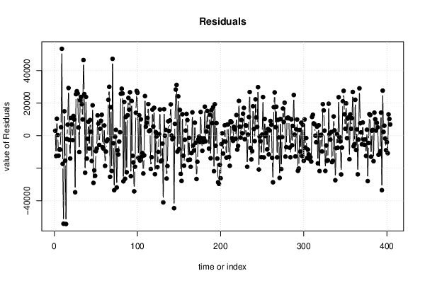
| Residual Standard Deviation | 1.631e+04 |
| Sum Squared Residuals | 1.016e+11 |
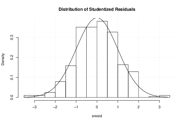
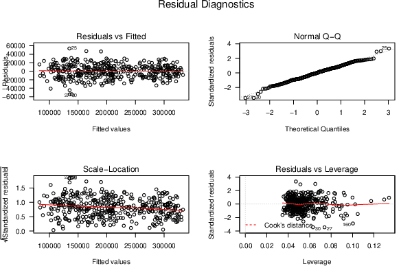
| Menu of Residual Diagnostics | |
| Description | Link |
| Histogram | Compute |
| Central Tendency | Compute |
| QQ Plot | Compute |
| Kernel Density Plot | Compute |
| Skewness/Kurtosis Test | Compute |
| Skewness-Kurtosis Plot | Compute |
| Harrell-Davis Plot | Compute |
| Bootstrap Plot -- Central Tendency | Compute |
| Blocked Bootstrap Plot -- Central Tendency | Compute |
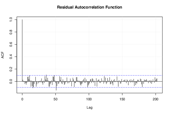
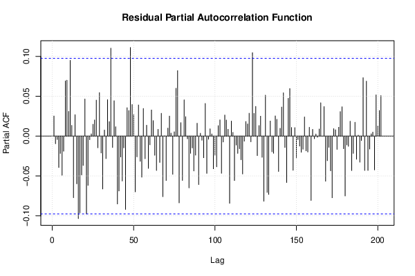
| (Partial) Autocorrelation Plot | Compute |
| Spectral Analysis | Compute |
| Tukey lambda PPCC Plot | Compute |
| Box-Cox Normality Plot | Compute |
| Summary Statistics | Compute |
| Ramsey RESET F-Test for powers (2 and 3) of fitted values |
> reset_test_fitted RESET test data: mylm RESET = 0.094702, df1 = 2, df2 = 380, p-value = 0.9097 |
| Ramsey RESET F-Test for powers (2 and 3) of regressors |
> reset_test_regressors RESET test data: mylm RESET = 0.61226, df1 = 42, df2 = 340, p-value = 0.973 |
| Ramsey RESET F-Test for powers (2 and 3) of principal components |
> reset_test_principal_components RESET test data: mylm RESET = 0.53392, df1 = 2, df2 = 380, p-value = 0.5867 |
| Variance Inflation Factors (Multicollinearity) |
> vif
               unit_price               defl_price1                       dum
                40.166900                 69.313475                 29.161236
              US_IND_PROD            defl_price1dum  `barrels_purchased(t-1)`
                49.312008                 57.704473                 18.159918
 `barrels_purchased(t-2)`  `barrels_purchased(t-3)` `barrels_purchased(t-1s)`
                17.637154                 17.495015                 12.292517
                       M1                        M2                        M3
                 2.255756                  2.077452                  2.081585
                       M4                        M5                        M6
                 2.064527                  2.112393                  2.136109
                       M7                        M8                        M9
                 1.995894                  2.126247                  1.924205
                      M10                       M11                         t
                 2.116145                  2.240650                 71.598963
|