Free Statistics
of Irreproducible Research!
Description of Statistical Computation | ||||||||||||||||||||||||||||||||||||||||||||||||||||||
|---|---|---|---|---|---|---|---|---|---|---|---|---|---|---|---|---|---|---|---|---|---|---|---|---|---|---|---|---|---|---|---|---|---|---|---|---|---|---|---|---|---|---|---|---|---|---|---|---|---|---|---|---|---|---|
| Author's title | ||||||||||||||||||||||||||||||||||||||||||||||||||||||
| Author | *The author of this computation has been verified* | |||||||||||||||||||||||||||||||||||||||||||||||||||||
| R Software Module | rwasp_bidensity.wasp | |||||||||||||||||||||||||||||||||||||||||||||||||||||
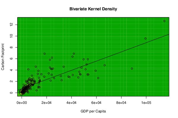
| Title produced by software | Bivariate Kernel Density Estimation | |||||||||||||||||||||||||||||||||||||||||||||||||||||
| Date of computation | Sun, 16 Dec 2018 18:10:19 +0100 | |||||||||||||||||||||||||||||||||||||||||||||||||||||
| Cite this page as follows | Statistical Computations at FreeStatistics.org, Office for Research Development and Education, URL https://freestatistics.org/blog/index.php?v=date/2018/Dec/16/t1544980403ksikzaqnlrmyvxj.htm/, Retrieved Sun, 05 May 2024 06:27:03 +0000 | |||||||||||||||||||||||||||||||||||||||||||||||||||||
| Statistical Computations at FreeStatistics.org, Office for Research Development and Education, URL https://freestatistics.org/blog/index.php?pk=315900, Retrieved Sun, 05 May 2024 06:27:03 +0000 | ||||||||||||||||||||||||||||||||||||||||||||||||||||||
| QR Codes: | ||||||||||||||||||||||||||||||||||||||||||||||||||||||
|
| ||||||||||||||||||||||||||||||||||||||||||||||||||||||
| Original text written by user: | ||||||||||||||||||||||||||||||||||||||||||||||||||||||
| IsPrivate? | No (this computation is public) | |||||||||||||||||||||||||||||||||||||||||||||||||||||
| User-defined keywords | ||||||||||||||||||||||||||||||||||||||||||||||||||||||
| Estimated Impact | 87 | |||||||||||||||||||||||||||||||||||||||||||||||||||||
Tree of Dependent Computations | ||||||||||||||||||||||||||||||||||||||||||||||||||||||
| Family? (F = Feedback message, R = changed R code, M = changed R Module, P = changed Parameters, D = changed Data) | ||||||||||||||||||||||||||||||||||||||||||||||||||||||
| - [Bivariate Kernel Density Estimation] [Countries 4] [2018-12-16 17:10:19] [e5fb83f5878d2d8e7ed5cb1b57a35a7d] [Current] | ||||||||||||||||||||||||||||||||||||||||||||||||||||||
| Feedback Forum | ||||||||||||||||||||||||||||||||||||||||||||||||||||||
Post a new message | ||||||||||||||||||||||||||||||||||||||||||||||||||||||
Dataset | ||||||||||||||||||||||||||||||||||||||||||||||||||||||
| Dataseries X: | ||||||||||||||||||||||||||||||||||||||||||||||||||||||
614.66 4534.37 5430.57 4665.91 13205.1 13540 3426.39 NA 66604.2 51274.1 7106.04 22647.3 24299 857.5 15722.8 6300.45 48053.3 746.83 70626.3 2395 2253.09 4708.85 7743.5 13237.6 NA 47097.4 7615.28 671.07 276.69 3801.45 877.64 1271.21 52145.4 NA 495.04 1161.22 14525.8 5560.94 7305.22 860.24 1943.69 338.63 8979.96 1016.83 14522.8 5175.94 31454.7 21676.3 61413.6 1433.17 7088.01 6085.89 5192.88 2930.33 3696.33 24064 439.73 17304.4 379.38 4201.37 50960.2 45430.3 NA NA 11989 505.76 3710.7 46822.4 1627.9 25987.4 7410.48 NA 3233.8 459.09 681.25 3269.46 749.13 2269.51 13964.2 1513.85 3688.53 7511.1 5848.54 52853.6 33718.9 38412 5226.3 46201.6 4615.17 11278 1062.11 NA 24155.8 41830.5 1116.37 1236.24 13732 9143.86 1338.42 397.38 5859.43 14373.7 114665 5174.89 456.33 493.84 10252.6 741.22 NA 1524.39 8811.15 10123.9 1971.03 3736.07 7251.6 NA 3149.43 538.82 1117.58 5880.8 NA 700.07 53589.9 NA 37488.3 1626.85 410.91 2612.12 100172 22622.8 1218.6 8410.77 1871.21 3557.31 5684.73 2379.44 13769.5 23217.3 99431.5 NA 9213.94 13320.2 628.08 12952.5 7737.2 6171.48 4067.15 1384.53 23593.8 1079.27 6426.18 499.89 53122.4 18103.1 25040.5 1647.86 NA 8089.87 32008.7 2880.03 8190.7 4657.48 59381.9 88506.2 NA 836.17 765.33 5479.29 5167.86 580.86 4330.9 18310.8 4305.07 10437.7 5290.14 601.35 3589.63 40980.5 40817.4 49725 14238.1 1560.85 10237.8 1532.31 NA 1302.3 1740.64 865.91 | ||||||||||||||||||||||||||||||||||||||||||||||||||||||
| Dataseries Y: | ||||||||||||||||||||||||||||||||||||||||||||||||||||||
0.18 0.87 1.14 0.2 NA 1.08 0.89 NA 4.85 4.14 1.25 4.46 6.19 0.26 3.28 2.57 4.43 0.51 NA 0.63 0.67 1.74 2.36 0.91 NA 3.24 2.08 0.12 0.04 NA NA 0.19 5 3.56 0.08 0.01 2.04 2.32 0.67 0.25 0.47 0.07 1.37 0.26 2.21 1.23 2.94 3.42 2.6 NA 1.47 0.86 1.08 1.02 0.84 3.17 0.03 NA 0.07 1.06 NA 2.71 1.58 2.39 0.43 0.21 0.83 3.28 0.43 2.58 NA 2.61 0.7 0.16 0.09 1.25 0.15 0.6 1.9 0.61 0.64 1.72 1.36 3.22 4.59 2.77 1.09 3.69 1.09 4.59 0.2 0.68 4.17 6.89 0.95 0.09 1.66 2.52 0.51 0.14 2.33 2.15 12.65 2.06 0.07 0.07 2.1 0.1 1.73 0.55 1.99 1.74 1.03 2.09 2.13 NA 0.67 0.17 0.09 1.02 NA 0.16 3.23 1.78 2.84 0.45 0.1 0.21 NA 5.8 0.38 1.44 0.35 0.97 0.67 0.34 2.64 2.15 9.57 3.27 1.46 3.87 0.07 3.34 1.56 NA 0.96 0.37 4.21 0.3 1.66 0.07 5.91 2.82 4.27 0 0.07 2.34 2.22 0.52 3.01 0.67 3.88 4.26 0.81 0.13 0.17 1.54 0.06 0.31 0.88 6.89 1.11 1.92 4.13 0.08 1.92 3.14 6.37 5.9 0.98 1.41 2.13 0.79 NA 0.42 0.24 0.53 | ||||||||||||||||||||||||||||||||||||||||||||||||||||||
Tables (Output of Computation) | ||||||||||||||||||||||||||||||||||||||||||||||||||||||
| ||||||||||||||||||||||||||||||||||||||||||||||||||||||
Figures (Output of Computation) | ||||||||||||||||||||||||||||||||||||||||||||||||||||||
Input Parameters & R Code | ||||||||||||||||||||||||||||||||||||||||||||||||||||||
| Parameters (Session): | ||||||||||||||||||||||||||||||||||||||||||||||||||||||
| par1 = grey ; par2 = no ; | ||||||||||||||||||||||||||||||||||||||||||||||||||||||
| Parameters (R input): | ||||||||||||||||||||||||||||||||||||||||||||||||||||||
| par1 = 50 ; par2 = 50 ; par3 = 0 ; par4 = 0 ; par5 = 0 ; par6 = Y ; par7 = Y ; par8 = terrain.colors ; | ||||||||||||||||||||||||||||||||||||||||||||||||||||||
| R code (references can be found in the software module): | ||||||||||||||||||||||||||||||||||||||||||||||||||||||
par1 <- as(par1,'numeric') | ||||||||||||||||||||||||||||||||||||||||||||||||||||||