| Multiple Linear Regression - Estimated Regression Equation |
| dPQ[t] = -1.05291 + 3.01624dM[t] + 0.503724dM1[t] -1.04033dM2[t] + 0.48741dM3[t] + 0.969687dGf[t] -2.31852dGf1[t] + 0.861168dGf2[t] + 2.19187dGf3[t] + e[t] |
| Multiple Linear Regression - Ordinary Least Squares | |||||
| Variable | Parameter | S.D. | T-STAT H0: parameter = 0 | 2-tail p-value | 1-tail p-value |
| (Intercept) | -1.053 | 0.9885 | -1.0650e+00 | 0.3017 | 0.1509 |
| dM | +3.016 | 1.022 | +2.9520e+00 | 0.008919 | 0.00446 |
| dM1 | +0.5037 | 1.202 | +4.1920e-01 | 0.6803 | 0.3402 |
| dM2 | -1.04 | 1.207 | -8.6200e-01 | 0.4007 | 0.2004 |
| dM3 | +0.4874 | 1.085 | +4.4910e-01 | 0.659 | 0.3295 |
| dGf | +0.9697 | 0.9288 | +1.0440e+00 | 0.3111 | 0.1555 |
| dGf1 | -2.318 | 1.313 | -1.7660e+00 | 0.09529 | 0.04764 |
| dGf2 | +0.8612 | 1.548 | +5.5640e-01 | 0.5852 | 0.2926 |
| dGf3 | +2.192 | 1.508 | +1.4540e+00 | 0.1642 | 0.08209 |
| Multiple Linear Regression - Regression Statistics | |
| Multiple R | 0.7783 |
| R-squared | 0.6058 |
| Adjusted R-squared | 0.4203 |
| F-TEST (value) | 3.265 |
| F-TEST (DF numerator) | 8 |
| F-TEST (DF denominator) | 17 |
| p-value | 0.01919 |
| Multiple Linear Regression - Residual Statistics | |
| Residual Standard Deviation | 2.677 |
| Sum Squared Residuals | 121.8 |
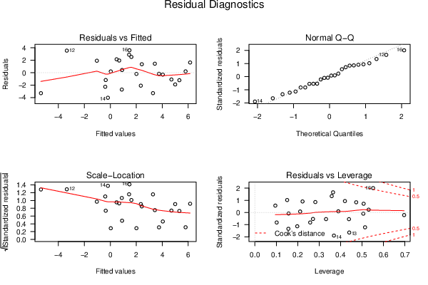
| Menu of Residual Diagnostics | |
| Description | Link |
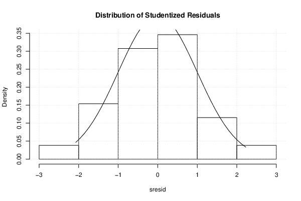
| Histogram | Compute |
| Central Tendency | Compute |
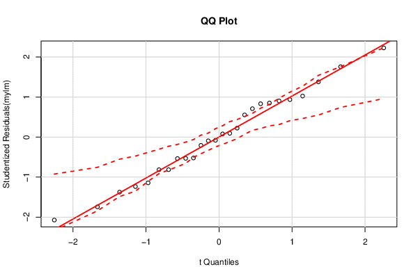
| QQ Plot | Compute |
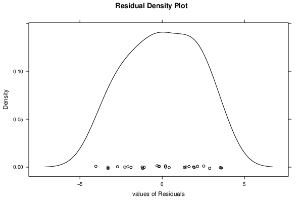
| Kernel Density Plot | Compute |
| Skewness/Kurtosis Test | Compute |
| Skewness-Kurtosis Plot | Compute |
| Harrell-Davis Plot | Compute |
| Bootstrap Plot -- Central Tendency | Compute |
| Blocked Bootstrap Plot -- Central Tendency | Compute |
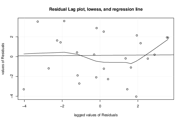
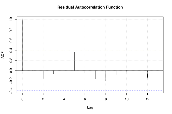
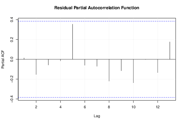
| (Partial) Autocorrelation Plot | Compute |
| Spectral Analysis | Compute |
| Tukey lambda PPCC Plot | Compute |
| Box-Cox Normality Plot | Compute |
| Summary Statistics | Compute |
| Multiple Linear Regression - Actuals, Interpolation, and Residuals | |||
| Time or Index | Actuals | Interpolation Forecast | Residuals Prediction Error |
| 1 | -0.01 | 3.285 | -3.295 |
| 2 | 4.87 | 3.43 | 1.44 |
| 3 | 0.26 | 2.349 | -2.088 |
| 4 | 1.81 | 2.012 | -0.2023 |
| 5 | 4.15 | 1.623 | 2.527 |
| 6 | 0.23 | 0.03565 | 0.1943 |
| 7 | 4.33 | 1.447 | 2.883 |
| 8 | 3.57 | 3.751 | -0.1806 |
| 9 | 3.78 | 2.427 | 1.353 |
| 10 | 2.63 | 0.4848 | 2.145 |
| 11 | 2.63 | 0.6838 | 1.946 |
| 12 | 0.19 | -3.35 | 3.54 |
| 13 | -8.64 | -5.342 | -3.298 |
| 14 | -4.22 | -0.1859 | -4.034 |
| 15 | 0.88 | -1.035 | 1.915 |
| 16 | 5.07 | 1.475 | 3.595 |
| 17 | 3.1 | 4.996 | -1.896 |
| 18 | -1.54 | -0.3525 | -1.187 |
| 19 | -1.83 | 0.8864 | -2.716 |
| 20 | 3.61 | 4.708 | -1.098 |
| 21 | 7.78 | 6.147 | 1.633 |
| 22 | -2.66 | -0.389 | -2.271 |
| 23 | 1.33 | 0.9071 | 0.4229 |
| 24 | 4.1 | 5.318 | -1.218 |
| 25 | 6 | 5.797 | 0.2032 |
| 26 | 3.73 | 4.043 | -0.3125 |
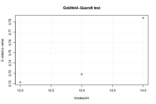
| Goldfeld-Quandt test for Heteroskedasticity | |||
| p-values | Alternative Hypothesis | ||
| breakpoint index | greater | 2-sided | less |
| 12 | 0.6394 | 0.7211 | 0.3606 |
| 13 | 0.6355 | 0.7289 | 0.3645 |
| 14 | 0.6081 | 0.7838 | 0.3919 |
| Meta Analysis of Goldfeld-Quandt test for Heteroskedasticity | |||
| Description | # significant tests | % significant tests | OK/NOK |
| 1% type I error level | 0 | 0 | OK |
| 5% type I error level | 0 | 0 | OK |
| 10% type I error level | 0 | 0 | OK |
| Ramsey RESET F-Test for powers (2 and 3) of fitted values |
> reset_test_fitted RESET test data: mylm RESET = 0.74891, df1 = 2, df2 = 15, p-value = 0.4898 |
| Ramsey RESET F-Test for powers (2 and 3) of regressors |
> reset_test_regressors RESET test data: mylm RESET = 0.3778, df1 = 16, df2 = 1, p-value = 0.8767 |
| Ramsey RESET F-Test for powers (2 and 3) of principal components |
> reset_test_principal_components RESET test data: mylm RESET = 0.43146, df1 = 2, df2 = 15, p-value = 0.6574 |
| Variance Inflation Factors (Multicollinearity) |
> vif
      dM      dM1      dM2      dM3      dGf     dGf1     dGf2     dGf3
2.054034 2.362136 2.213141 1.721041 1.813697 1.699729 1.143829 1.214966
|