| Multiple Linear Regression - Estimated Regression Equation |
| a[t] = + 1.62354 + 0.0280908b[t] + 0.0374991c[t] -0.0695361d[t] + 0.143442e[t] + 0.282583f[t] -0.042036g[t] + 0.0865618h[t] -0.034961i[t] -0.0547529j[t] + e[t] |
| Multiple Linear Regression - Ordinary Least Squares | |||||
| Variable | Parameter | S.D. | T-STAT H0: parameter = 0 | 2-tail p-value | 1-tail p-value |
| (Intercept) | +1.623 | 3.185 | +5.0980e-01 | 0.6167 | 0.3084 |
| b | +0.02809 | 0.2102 | +1.3370e-01 | 0.8952 | 0.4476 |
| c | +0.0375 | 0.0604 | +6.2090e-01 | 0.5429 | 0.2715 |
| d | -0.06954 | 0.3156 | -2.2030e-01 | 0.8282 | 0.4141 |
| e | +0.1434 | 0.2114 | +6.7840e-01 | 0.5066 | 0.2533 |
| f | +0.2826 | 0.2158 | +1.3090e+00 | 0.2079 | 0.1039 |
| g | -0.04204 | 0.02789 | -1.5070e+00 | 0.1501 | 0.07506 |
| h | +0.08656 | 0.2168 | +3.9930e-01 | 0.6947 | 0.3473 |
| i | -0.03496 | 0.3207 | -1.0900e-01 | 0.9145 | 0.4572 |
| j | -0.05475 | 0.2455 | -2.2300e-01 | 0.8262 | 0.4131 |
| Multiple Linear Regression - Regression Statistics | |
| Multiple R | 0.5051 |
| R-squared | 0.2552 |
| Adjusted R-squared | -0.1392 |
| F-TEST (value) | 0.6471 |
| F-TEST (DF numerator) | 9 |
| F-TEST (DF denominator) | 17 |
| p-value | 0.7432 |
| Multiple Linear Regression - Residual Statistics | |
| Residual Standard Deviation | 0.4766 |
| Sum Squared Residuals | 3.862 |
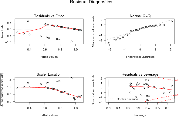
| Menu of Residual Diagnostics | |
| Description | Link |
| Histogram | Compute |
| Central Tendency | Compute |
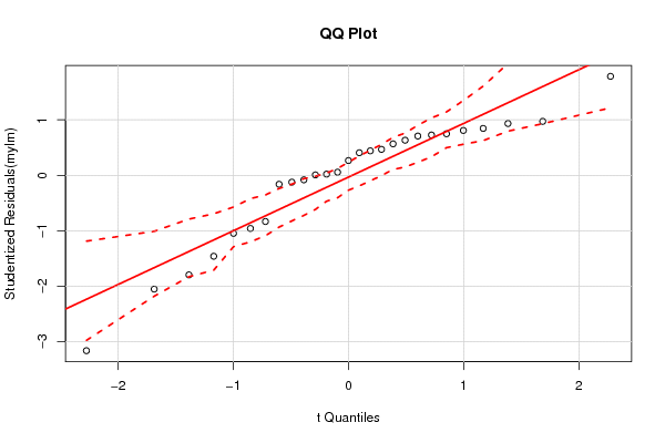
| QQ Plot | Compute |
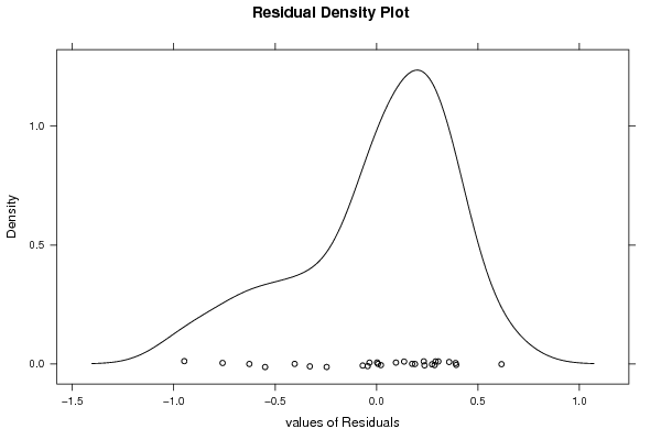
| Kernel Density Plot | Compute |
| Skewness/Kurtosis Test | Compute |
| Skewness-Kurtosis Plot | Compute |
| Harrell-Davis Plot | Compute |
| Bootstrap Plot -- Central Tendency | Compute |
| Blocked Bootstrap Plot -- Central Tendency | Compute |
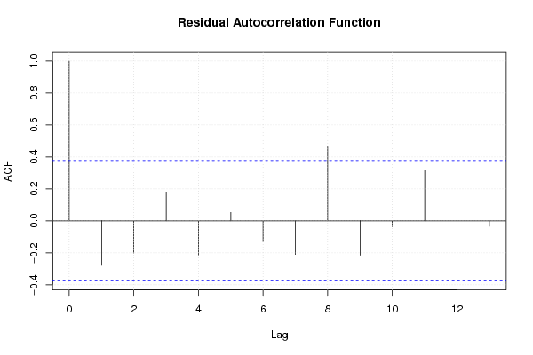
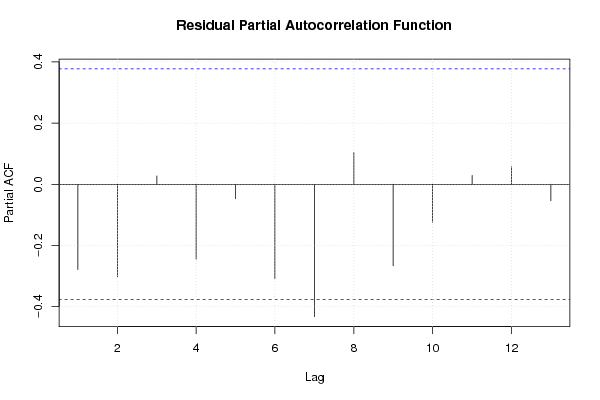
| (Partial) Autocorrelation Plot | Compute |
| Spectral Analysis | Compute |
| Tukey lambda PPCC Plot | Compute |
| Box-Cox Normality Plot | Compute |
| Summary Statistics | Compute |
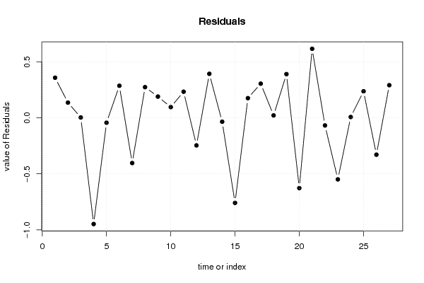
| Multiple Linear Regression - Actuals, Interpolation, and Residuals | |||
| Time or Index | Actuals | Interpolation Forecast | Residuals Prediction Error |
| 1 | 1 | 0.6421 | 0.3579 |
| 2 | 1 | 0.8642 | 0.1358 |
| 3 | 1 | 0.9971 | 0.002887 |
| 4 | 0 | 0.9479 | -0.9479 |
| 5 | 1 | 1.044 | -0.04363 |
| 6 | 1 | 0.7139 | 0.2861 |
| 7 | 0 | 0.4036 | -0.4036 |
| 8 | 1 | 0.7265 | 0.2735 |
| 9 | 1 | 0.8106 | 0.1894 |
| 10 | 1 | 0.9043 | 0.09565 |
| 11 | 1 | 0.7671 | 0.2329 |
| 12 | 0 | 0.2461 | -0.2461 |
| 13 | 1 | 0.6074 | 0.3926 |
| 14 | 1 | 1.035 | -0.03477 |
| 15 | 0 | 0.7591 | -0.7591 |
| 16 | 1 | 0.8246 | 0.1754 |
| 17 | 1 | 0.6954 | 0.3046 |
| 18 | 1 | 0.9786 | 0.02144 |
| 19 | 1 | 0.6101 | 0.3899 |
| 20 | 0 | 0.6271 | -0.6271 |
| 21 | 1 | 0.384 | 0.616 |
| 22 | 1 | 1.068 | -0.06823 |
| 23 | 0 | 0.5494 | -0.5494 |
| 24 | 1 | 0.993 | 0.006969 |
| 25 | 1 | 0.7633 | 0.2367 |
| 26 | 0 | 0.3289 | -0.3289 |
| 27 | 1 | 0.709 | 0.291 |
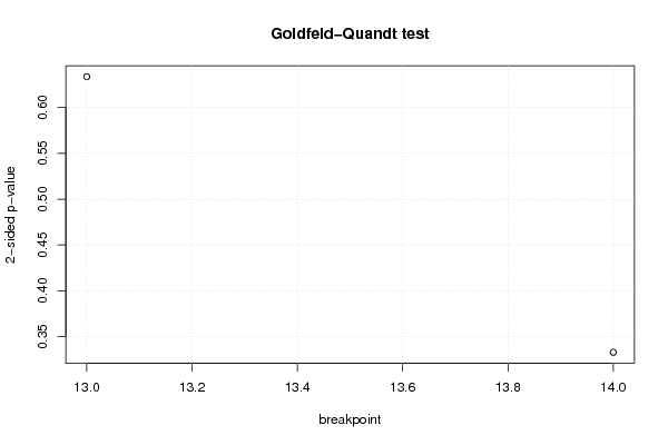
| Goldfeld-Quandt test for Heteroskedasticity | |||
| p-values | Alternative Hypothesis | ||
| breakpoint index | greater | 2-sided | less |
| 13 | 0.3168 | 0.6336 | 0.6832 |
| 14 | 0.1665 | 0.3329 | 0.8335 |
| Meta Analysis of Goldfeld-Quandt test for Heteroskedasticity | |||
| Description | # significant tests | % significant tests | OK/NOK |
| 1% type I error level | 0 | 0 | OK |
| 5% type I error level | 0 | 0 | OK |
| 10% type I error level | 0 | 0 | OK |
| Ramsey RESET F-Test for powers (2 and 3) of fitted values |
> reset_test_fitted RESET test data: mylm RESET = 0.66139, df1 = 2, df2 = 15, p-value = 0.5306 |
| Ramsey RESET F-Test for powers (2 and 3) of regressors |
> reset_test_regressors RESET test data: mylm RESET = -0.091511, df1 = 18, df2 = -1, p-value = NA |
| Ramsey RESET F-Test for powers (2 and 3) of principal components |
> reset_test_principal_components RESET test data: mylm RESET = 0.025121, df1 = 2, df2 = 15, p-value = 0.9752 |
| Variance Inflation Factors (Multicollinearity) |
> vif
       b        c        d        e        f        g        h        i
1.166443 1.282110 1.493951 1.311818 1.245430 1.335541 1.302755 1.547351
       j
1.493378
|