| Multiple Linear Regression - Estimated Regression Equation |
| a[t] = + 1.75911 + 0.167728b[t] + 0.00629334c[t] -0.0307333d[t] -0.153297e[t] -0.00937832f[t] -0.0255257g[t] -0.180189h[t] + 0.0367055i[t] + 0.420593j[t] + e[t] |
| Multiple Linear Regression - Ordinary Least Squares | |||||
| Variable | Parameter | S.D. | T-STAT H0: parameter = 0 | 2-tail p-value | 1-tail p-value |
| (Intercept) | +1.759 | 2.683 | +6.5570e-01 | 0.5185 | 0.2593 |
| b | +0.1677 | 0.1907 | +8.7940e-01 | 0.3883 | 0.1941 |
| c | +0.006293 | 0.0577 | +1.0910e-01 | 0.9141 | 0.457 |
| d | -0.03073 | 0.2641 | -1.1640e-01 | 0.9084 | 0.4542 |
| e | -0.1533 | 0.2191 | -6.9970e-01 | 0.4911 | 0.2456 |
| f | -0.009378 | 0.06777 | -1.3840e-01 | 0.8911 | 0.4456 |
| g | -0.02553 | 0.03343 | -7.6360e-01 | 0.4528 | 0.2264 |
| h | -0.1802 | 0.2175 | -8.2830e-01 | 0.416 | 0.208 |
| i | +0.03671 | 0.271 | +1.3550e-01 | 0.8934 | 0.4467 |
| j | +0.4206 | 0.201 | +2.0930e+00 | 0.04761 | 0.02381 |
| Multiple Linear Regression - Regression Statistics | |
| Multiple R | 0.5086 |
| R-squared | 0.2587 |
| Adjusted R-squared | -0.03139 |
| F-TEST (value) | 0.8918 |
| F-TEST (DF numerator) | 9 |
| F-TEST (DF denominator) | 23 |
| p-value | 0.5473 |
| Multiple Linear Regression - Residual Statistics | |
| Residual Standard Deviation | 0.4862 |
| Sum Squared Residuals | 5.436 |
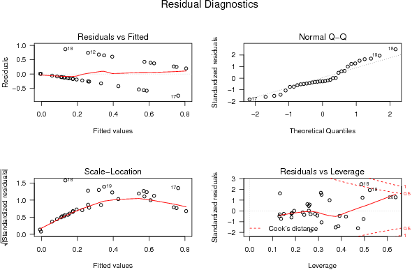
| Menu of Residual Diagnostics | |
| Description | Link |
| Histogram | Compute |
| Central Tendency | Compute |
| QQ Plot | Compute |
| Kernel Density Plot | Compute |
| Skewness/Kurtosis Test | Compute |
| Skewness-Kurtosis Plot | Compute |
| Harrell-Davis Plot | Compute |
| Bootstrap Plot -- Central Tendency | Compute |
| Blocked Bootstrap Plot -- Central Tendency | Compute |
| (Partial) Autocorrelation Plot | Compute |
| Spectral Analysis | Compute |
| Tukey lambda PPCC Plot | Compute |
| Box-Cox Normality Plot | Compute |
| Summary Statistics | Compute |
| Multiple Linear Regression - Actuals, Interpolation, and Residuals | |||
| Time or Index | Actuals | Interpolation Forecast | Residuals Prediction Error |
| 1 | 1 | 0.5739 | 0.4261 |
| 2 | 0 | 0.1753 | -0.1753 |
| 3 | 1 | 0.3198 | 0.6802 |
| 4 | 0 | 0.2273 | -0.2273 |
| 5 | 1 | 0.7379 | 0.2621 |
| 6 | 0 | 0.1252 | -0.1252 |
| 7 | 0 | 0.1472 | -0.1472 |
| 8 | 1 | 0.8067 | 0.1933 |
| 9 | 0 | 0.332 | -0.332 |
| 10 | 0 | 0.1291 | -0.1291 |
| 11 | 0 | 0.1959 | -0.1959 |
| 12 | 1 | 0.2594 | 0.7406 |
| 13 | 1 | 0.3945 | 0.6056 |
| 14 | 1 | 0.7531 | 0.2469 |
| 15 | 1 | 0.6083 | 0.3917 |
| 16 | 0 | 0.5701 | -0.5701 |
| 17 | 0 | 0.7624 | -0.7624 |
| 18 | 1 | 0.1331 | 0.8669 |
| 19 | 1 | 0.3493 | 0.6507 |
| 20 | 1 | 0.6279 | 0.3721 |
| 21 | 0 | -0.008099 | 0.008099 |
| 22 | 0 | -0.002868 | 0.002868 |
| 23 | 0 | 0.5867 | -0.5867 |
| 24 | 0 | 0.1089 | -0.1089 |
| 25 | 0 | 0.1559 | -0.1559 |
| 26 | 0 | 0.1143 | -0.1143 |
| 27 | 0 | 0.08657 | -0.08657 |
| 28 | 0 | 0.1741 | -0.1741 |
| 29 | 0 | 0.2657 | -0.2657 |
| 30 | 0 | 0.5431 | -0.5431 |
| 31 | 0 | 0.05903 | -0.05903 |
| 32 | 0 | 0.4286 | -0.4286 |
| 33 | 0 | 0.2598 | -0.2598 |
| Goldfeld-Quandt test for Heteroskedasticity | |||
| p-values | Alternative Hypothesis | ||
| breakpoint index | greater | 2-sided | less |
| 13 | 0.4688 | 0.9375 | 0.5312 |
| 14 | 0.8209 | 0.3582 | 0.1791 |
| 15 | 0.8529 | 0.2941 | 0.1471 |
| 16 | 0.9591 | 0.08185 | 0.04092 |
| 17 | 0.932 | 0.136 | 0.06798 |
| 18 | 0.9943 | 0.01134 | 0.005672 |
| 19 | 0.9995 | 0.001049 | 0.0005247 |
| 20 | 1 | 0 | 0 |
| Meta Analysis of Goldfeld-Quandt test for Heteroskedasticity | |||
| Description | # significant tests | % significant tests | OK/NOK |
| 1% type I error level | 2 | 0.25 | NOK |
| 5% type I error level | 3 | 0.375 | NOK |
| 10% type I error level | 4 | 0.5 | NOK |
| Ramsey RESET F-Test for powers (2 and 3) of fitted values |
> reset_test_fitted RESET test data: mylm RESET = 0.16347, df1 = 2, df2 = 21, p-value = 0.8503 |
| Ramsey RESET F-Test for powers (2 and 3) of regressors |
> reset_test_regressors RESET test data: mylm RESET = 0.25138, df1 = 18, df2 = 5, p-value = 0.9868 |
| Ramsey RESET F-Test for powers (2 and 3) of principal components |
> reset_test_principal_components RESET test data: mylm RESET = 2.0522, df1 = 2, df2 = 21, p-value = 0.1534 |
| Variance Inflation Factors (Multicollinearity) |
> vif
       b        c        d        e        f        g        h        i
1.259231 1.559793 1.251869 1.415288 1.347087 1.351416 1.310398 1.307410
       j
1.118705
|