| Multiple Linear Regression - Estimated Regression Equation |
| A[t] = + 1.9793 + 0.347087B[t] + 0.0102604C[t] -1.34422D[t] -1.15675E[t] -1.25826F[t] -0.582743G[t] -0.0673211H[t] -0.0232844I[t] -0.00238079J[t] -0.0239932K[t] -0.151998L[t] + 0.419445M[t] + e[t] |
| Multiple Linear Regression - Ordinary Least Squares | |||||
| Variable | Parameter | S.D. | T-STAT H0: parameter = 0 | 2-tail p-value | 1-tail p-value |
| (Intercept) | +1.979 | 1.639 | +1.2070e+00 | 0.2414 | 0.1207 |
| B | +0.3471 | 0.2167 | +1.6010e+00 | 0.125 | 0.06248 |
| C | +0.01026 | 0.05827 | +1.7610e-01 | 0.862 | 0.431 |
| D | -1.344 | 0.5316 | -2.5290e+00 | 0.01997 | 0.009985 |
| E | -1.157 | 0.6719 | -1.7220e+00 | 0.1006 | 0.0503 |
| F | -1.258 | 0.506 | -2.4860e+00 | 0.02186 | 0.01093 |
| G | -0.5827 | 0.3475 | -1.6770e+00 | 0.1091 | 0.05456 |
| H | -0.06732 | 0.2292 | -2.9370e-01 | 0.772 | 0.386 |
| I | -0.02328 | 0.06565 | -3.5470e-01 | 0.7265 | 0.3633 |
| J | -0.002381 | 0.008294 | -2.8700e-01 | 0.777 | 0.3885 |
| K | -0.02399 | 0.2046 | -1.1720e-01 | 0.9078 | 0.4539 |
| L | -0.152 | 0.2743 | -5.5400e-01 | 0.5857 | 0.2928 |
| M | +0.4194 | 0.1923 | +2.1810e+00 | 0.04128 | 0.02064 |
| Multiple Linear Regression - Regression Statistics | |
| Multiple R | 0.6619 |
| R-squared | 0.4381 |
| Adjusted R-squared | 0.1009 |
| F-TEST (value) | 1.299 |
| F-TEST (DF numerator) | 12 |
| F-TEST (DF denominator) | 20 |
| p-value | 0.2921 |
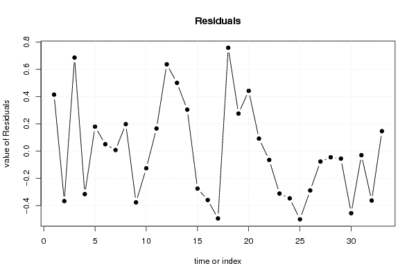
| Multiple Linear Regression - Residual Statistics | |
| Residual Standard Deviation | 0.4539 |
| Sum Squared Residuals | 4.121 |
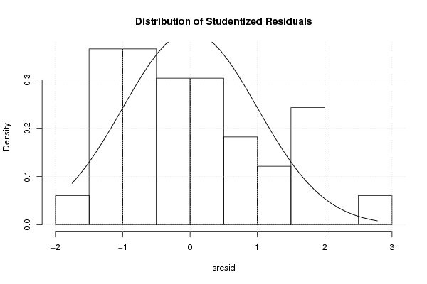
| Menu of Residual Diagnostics | |
| Description | Link |
| Histogram | Compute |
| Central Tendency | Compute |
| QQ Plot | Compute |
| Kernel Density Plot | Compute |
| Skewness/Kurtosis Test | Compute |
| Skewness-Kurtosis Plot | Compute |
| Harrell-Davis Plot | Compute |
| Bootstrap Plot -- Central Tendency | Compute |
| Blocked Bootstrap Plot -- Central Tendency | Compute |
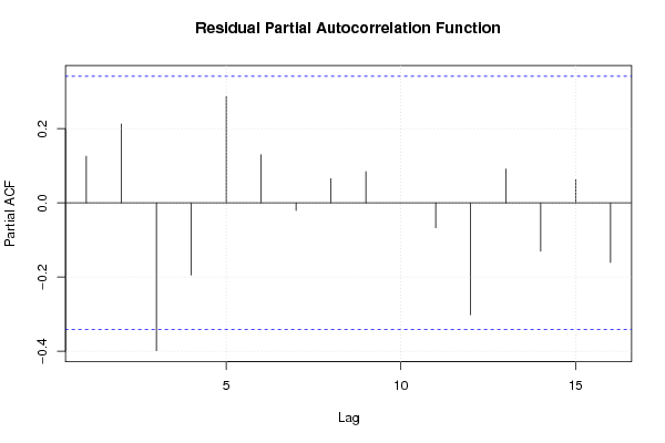
| (Partial) Autocorrelation Plot | Compute |
| Spectral Analysis | Compute |
| Tukey lambda PPCC Plot | Compute |
| Box-Cox Normality Plot | Compute |
| Summary Statistics | Compute |
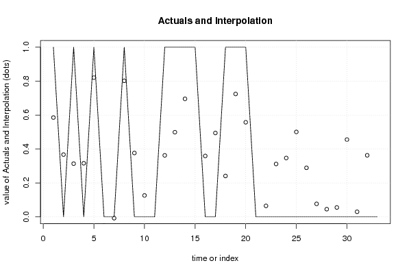
| Multiple Linear Regression - Actuals, Interpolation, and Residuals | |||
| Time or Index | Actuals | Interpolation Forecast | Residuals Prediction Error |
| 1 | 1 | 0.5856 | 0.4144 |
| 2 | 0 | 0.3672 | -0.3672 |
| 3 | 1 | 0.3138 | 0.6862 |
| 4 | 0 | 0.3161 | -0.3161 |
| 5 | 1 | 0.8209 | 0.1791 |
| 6 | 0 | -0.05042 | 0.05042 |
| 7 | 0 | -0.007508 | 0.007508 |
| 8 | 1 | 0.8022 | 0.1978 |
| 9 | 0 | 0.3768 | -0.3768 |
| 10 | 0 | 0.1265 | -0.1265 |
| 11 | 0 | -0.1657 | 0.1657 |
| 12 | 1 | 0.3628 | 0.6372 |
| 13 | 1 | 0.4992 | 0.5008 |
| 14 | 1 | 0.6958 | 0.3042 |
| 15 | 1 | 1.275 | -0.2754 |
| 16 | 0 | 0.3593 | -0.3593 |
| 17 | 0 | 0.4947 | -0.4947 |
| 18 | 1 | 0.2413 | 0.7587 |
| 19 | 1 | 0.7246 | 0.2754 |
| 20 | 1 | 0.5576 | 0.4424 |
| 21 | 0 | -0.09152 | 0.09152 |
| 22 | 0 | 0.0651 | -0.0651 |
| 23 | 0 | 0.3119 | -0.3119 |
| 24 | 0 | 0.3471 | -0.3471 |
| 25 | 0 | 0.5008 | -0.5008 |
| 26 | 0 | 0.2893 | -0.2893 |
| 27 | 0 | 0.07695 | -0.07695 |
| 28 | 0 | 0.04553 | -0.04553 |
| 29 | 0 | 0.05565 | -0.05565 |
| 30 | 0 | 0.4559 | -0.4559 |
| 31 | 0 | 0.03018 | -0.03018 |
| 32 | 0 | 0.3631 | -0.3631 |
| 33 | 0 | -0.1462 | 0.1462 |
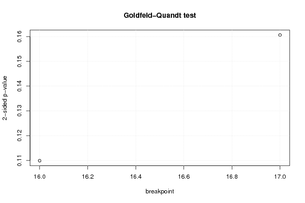
| Goldfeld-Quandt test for Heteroskedasticity | |||
| p-values | Alternative Hypothesis | ||
| breakpoint index | greater | 2-sided | less |
| 16 | 0.9451 | 0.1099 | 0.05494 |
| 17 | 0.9197 | 0.1607 | 0.08033 |
| Meta Analysis of Goldfeld-Quandt test for Heteroskedasticity | |||
| Description | # significant tests | % significant tests | OK/NOK |
| 1% type I error level | 0 | 0 | OK |
| 5% type I error level | 0 | 0 | OK |
| 10% type I error level | 0 | 0 | OK |
| Ramsey RESET F-Test for powers (2 and 3) of fitted values |
> reset_test_fitted RESET test data: mylm RESET = 2.2809, df1 = 2, df2 = 18, p-value = 0.1309 |
| Ramsey RESET F-Test for powers (2 and 3) of regressors |
> reset_test_regressors RESET test data: mylm RESET = -0.19354, df1 = 24, df2 = -4, p-value = NA |
| Ramsey RESET F-Test for powers (2 and 3) of principal components |
> reset_test_principal_components RESET test data: mylm RESET = 2.0433, df1 = 2, df2 = 18, p-value = 0.1586 |
| Variance Inflation Factors (Multicollinearity) |
> vif
        B         C         D         E         F         G         H         I
 1.865339  1.824621 10.057789  4.117072  6.854740  2.486593  1.777055  1.450285
        J         K         L         M
 1.276798  1.330293  1.537220  1.174726
|