Repository of Reproducible Computations

Free Statistics

of Irreproducible Research!

Author's title

Author

*Unverified author*

R Software Module

rwasp_decompose.wasp

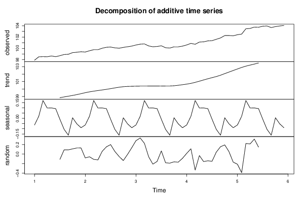
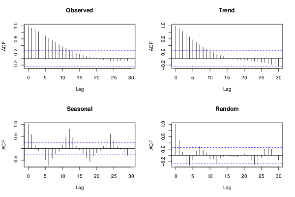
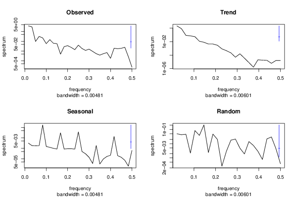
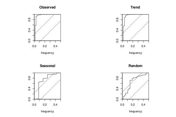
Title produced by software

Classical Decomposition

Date of computation

Mon, 01 May 2017 12:53:15 +0100

Cite this page as follows

Statistical Computations at FreeStatistics.org, Office for Research Development and Education, URL https://freestatistics.org/blog/index.php?v=date/2017/May/01/t149364057663i6ju7xicmmwi5.htm/, Retrieved Wed, 15 May 2024 22:25:17 +0200

Statistical Computations at FreeStatistics.org, Office for Research Development and Education, URL https://freestatistics.org/blog/index.php?pk=, Retrieved Wed, 15 May 2024 22:25:17 +0200

QR Codes:

Paste this QR Code to cite your computation.

Original text written by user:

IsPrivate?

No (this computation is public)

User-defined keywords

Estimated Impact

Dataseries X:

Download CSV

Histogram

Boxplots

Summary of computational transaction
Raw Input	view raw input (R code)
Raw Output	view raw output of R engine
Computing time	3 seconds
R Server	'Herman Ole Andreas Wold' @ wold.wessa.net

\begin{tabular}{lllllllll}
\hline
Summary of computational transaction \tabularnewline
Raw Input & view raw input (R code)  \tabularnewline
Raw Output & view raw output of R engine  \tabularnewline
Computing time & 3 seconds \tabularnewline
R Server & 'Herman Ole Andreas Wold' @ wold.wessa.net \tabularnewline
\hline
\end{tabular}
%Source: https://freestatistics.org/blog/index.php?pk=&T=0

[TABLE]
[ROW][C]Summary of computational transaction[/C][/ROW]
[ROW][C]Raw Input[/C][C]view raw input (R code) [/C][/ROW]
[ROW][C]Raw Output[/C][C]view raw output of R engine [/C][/ROW]
[ROW][C]Computing time[/C][C]3 seconds[/C][/ROW]
[ROW][C]R Server[/C][C]'Herman Ole Andreas Wold' @ wold.wessa.net[/C][/ROW]
[/TABLE]
Source: https://freestatistics.org/blog/index.php?pk=&T=0

Globally Unique Identifier (entire table): ba.freestatistics.org/blog/index.php?pk=&T=0

As an alternative you can also use a QR Code:

The GUIDs for individual cells are displayed in the table below:

Summary of computational transaction
Raw Input	view raw input (R code)
Raw Output	view raw output of R engine
Computing time	3 seconds
R Server	'Herman Ole Andreas Wold' @ wold.wessa.net

Classical Decomposition by Moving Averages
t	Observations	Fit	Trend	Seasonal	Random
1	97.91	NA	NA	-0.0638542	NA
2	98.51	NA	NA	0.0191667	NA
3	98.54	NA	NA	0.169896	NA
4	98.52	NA	NA	0.0977083	NA
5	98.66	NA	NA	0.09875	NA
6	98.53	NA	NA	0.0919792	NA
7	98.71	98.8212	98.8304	-0.00916667	-0.11125
8	98.92	98.8299	98.9354	-0.105521	0.0901042
9	98.96	98.87	99.0312	-0.16125	0.09
10	99.25	99.1398	99.1346	0.00520833	0.110208
11	99.32	99.191	99.2437	-0.0527083	0.128958
12	99.41	99.2802	99.3704	-0.0902083	0.129792
13	99.36	99.4399	99.5037	-0.0638542	-0.0798958
14	99.58	99.6358	99.6167	0.0191667	-0.0558333
15	99.77	99.8803	99.7104	0.169896	-0.110312
16	99.77	99.8915	99.7938	0.0977083	-0.121458
17	100.03	99.9717	99.8729	0.09875	0.0583333
18	100.2	100.047	99.955	0.0919792	0.153021
19	100.24	100.039	100.048	-0.00916667	0.200833
20	100.1	100.043	100.149	-0.105521	0.0567708
21	100.03	100.079	100.24	-0.16125	-0.04875
22	100.18	100.316	100.31	0.00520833	-0.135625
23	100.29	100.296	100.349	-0.0527083	-0.00645833
24	100.41	100.276	100.366	-0.0902083	0.134375
25	100.6	100.317	100.381	-0.0638542	0.283021
26	100.75	100.41	100.391	0.0191667	0.34
27	100.79	100.563	100.393	0.169896	0.227187
28	100.44	100.496	100.398	0.0977083	-0.0560417
29	100.29	100.501	100.402	0.09875	-0.210833
30	100.34	100.493	100.401	0.0919792	-0.153229
31	100.46	100.392	100.401	-0.00916667	0.0679167
32	100.12	100.302	100.408	-0.105521	-0.181979
33	100.06	100.25	100.411	-0.16125	-0.189583
34	100.28	100.442	100.437	0.00520833	-0.161875
35	100.28	100.449	100.501	-0.0527083	-0.168542
36	100.4	100.489	100.579	-0.0902083	-0.0885417
37	100.61	100.594	100.658	-0.0638542	0.0159375
38	100.89	100.777	100.758	0.0191667	0.112917
39	100.73	101.064	100.895	0.169896	-0.334479
40	101.12	101.15	101.052	0.0977083	-0.0297917
41	101.16	101.317	101.218	0.09875	-0.157083
42	101.33	101.47	101.378	0.0919792	-0.139896
43	101.37	101.52	101.53	-0.00916667	-0.150417
44	101.61	101.568	101.673	-0.105521	0.0421875
45	101.85	101.695	101.856	-0.16125	0.155417
46	102.27	102.076	102.07	0.00520833	0.194375
47	102.28	102.227	102.28	-0.0527083	0.053125
48	102.23	102.399	102.489	-0.0902083	-0.168542
49	102.42	102.632	102.696	-0.0638542	-0.211979
50	102.53	102.92	102.901	0.0191667	-0.39
51	103.47	103.245	103.075	0.169896	0.224688
52	103.53	103.316	103.218	0.0977083	0.214375
53	103.77	103.453	103.355	0.09875	0.316667
54	103.74	103.593	103.501	0.0919792	0.147188
55	103.93	NA	NA	-0.00916667	NA
56	103.97	NA	NA	-0.105521	NA
57	103.68	NA	NA	-0.16125	NA
58	103.86	NA	NA	0.00520833	NA
59	103.97	NA	NA	-0.0527083	NA
60	104.05	NA	NA	-0.0902083	NA

\begin{tabular}{lllllllll}
\hline
Classical Decomposition by Moving Averages \tabularnewline
t & Observations & Fit & Trend & Seasonal & Random \tabularnewline
1 & 97.91 & NA & NA & -0.0638542 & NA \tabularnewline
2 & 98.51 & NA & NA & 0.0191667 & NA \tabularnewline
3 & 98.54 & NA & NA & 0.169896 & NA \tabularnewline
4 & 98.52 & NA & NA & 0.0977083 & NA \tabularnewline
5 & 98.66 & NA & NA & 0.09875 & NA \tabularnewline
6 & 98.53 & NA & NA & 0.0919792 & NA \tabularnewline
7 & 98.71 & 98.8212 & 98.8304 & -0.00916667 & -0.11125 \tabularnewline
8 & 98.92 & 98.8299 & 98.9354 & -0.105521 & 0.0901042 \tabularnewline
9 & 98.96 & 98.87 & 99.0312 & -0.16125 & 0.09 \tabularnewline
10 & 99.25 & 99.1398 & 99.1346 & 0.00520833 & 0.110208 \tabularnewline
11 & 99.32 & 99.191 & 99.2437 & -0.0527083 & 0.128958 \tabularnewline
12 & 99.41 & 99.2802 & 99.3704 & -0.0902083 & 0.129792 \tabularnewline
13 & 99.36 & 99.4399 & 99.5037 & -0.0638542 & -0.0798958 \tabularnewline
14 & 99.58 & 99.6358 & 99.6167 & 0.0191667 & -0.0558333 \tabularnewline
15 & 99.77 & 99.8803 & 99.7104 & 0.169896 & -0.110312 \tabularnewline
16 & 99.77 & 99.8915 & 99.7938 & 0.0977083 & -0.121458 \tabularnewline
17 & 100.03 & 99.9717 & 99.8729 & 0.09875 & 0.0583333 \tabularnewline
18 & 100.2 & 100.047 & 99.955 & 0.0919792 & 0.153021 \tabularnewline
19 & 100.24 & 100.039 & 100.048 & -0.00916667 & 0.200833 \tabularnewline
20 & 100.1 & 100.043 & 100.149 & -0.105521 & 0.0567708 \tabularnewline
21 & 100.03 & 100.079 & 100.24 & -0.16125 & -0.04875 \tabularnewline
22 & 100.18 & 100.316 & 100.31 & 0.00520833 & -0.135625 \tabularnewline
23 & 100.29 & 100.296 & 100.349 & -0.0527083 & -0.00645833 \tabularnewline
24 & 100.41 & 100.276 & 100.366 & -0.0902083 & 0.134375 \tabularnewline
25 & 100.6 & 100.317 & 100.381 & -0.0638542 & 0.283021 \tabularnewline
26 & 100.75 & 100.41 & 100.391 & 0.0191667 & 0.34 \tabularnewline
27 & 100.79 & 100.563 & 100.393 & 0.169896 & 0.227187 \tabularnewline
28 & 100.44 & 100.496 & 100.398 & 0.0977083 & -0.0560417 \tabularnewline
29 & 100.29 & 100.501 & 100.402 & 0.09875 & -0.210833 \tabularnewline
30 & 100.34 & 100.493 & 100.401 & 0.0919792 & -0.153229 \tabularnewline
31 & 100.46 & 100.392 & 100.401 & -0.00916667 & 0.0679167 \tabularnewline
32 & 100.12 & 100.302 & 100.408 & -0.105521 & -0.181979 \tabularnewline
33 & 100.06 & 100.25 & 100.411 & -0.16125 & -0.189583 \tabularnewline
34 & 100.28 & 100.442 & 100.437 & 0.00520833 & -0.161875 \tabularnewline
35 & 100.28 & 100.449 & 100.501 & -0.0527083 & -0.168542 \tabularnewline
36 & 100.4 & 100.489 & 100.579 & -0.0902083 & -0.0885417 \tabularnewline
37 & 100.61 & 100.594 & 100.658 & -0.0638542 & 0.0159375 \tabularnewline
38 & 100.89 & 100.777 & 100.758 & 0.0191667 & 0.112917 \tabularnewline
39 & 100.73 & 101.064 & 100.895 & 0.169896 & -0.334479 \tabularnewline
40 & 101.12 & 101.15 & 101.052 & 0.0977083 & -0.0297917 \tabularnewline
41 & 101.16 & 101.317 & 101.218 & 0.09875 & -0.157083 \tabularnewline
42 & 101.33 & 101.47 & 101.378 & 0.0919792 & -0.139896 \tabularnewline
43 & 101.37 & 101.52 & 101.53 & -0.00916667 & -0.150417 \tabularnewline
44 & 101.61 & 101.568 & 101.673 & -0.105521 & 0.0421875 \tabularnewline
45 & 101.85 & 101.695 & 101.856 & -0.16125 & 0.155417 \tabularnewline
46 & 102.27 & 102.076 & 102.07 & 0.00520833 & 0.194375 \tabularnewline
47 & 102.28 & 102.227 & 102.28 & -0.0527083 & 0.053125 \tabularnewline
48 & 102.23 & 102.399 & 102.489 & -0.0902083 & -0.168542 \tabularnewline
49 & 102.42 & 102.632 & 102.696 & -0.0638542 & -0.211979 \tabularnewline
50 & 102.53 & 102.92 & 102.901 & 0.0191667 & -0.39 \tabularnewline
51 & 103.47 & 103.245 & 103.075 & 0.169896 & 0.224688 \tabularnewline
52 & 103.53 & 103.316 & 103.218 & 0.0977083 & 0.214375 \tabularnewline
53 & 103.77 & 103.453 & 103.355 & 0.09875 & 0.316667 \tabularnewline
54 & 103.74 & 103.593 & 103.501 & 0.0919792 & 0.147188 \tabularnewline
55 & 103.93 & NA & NA & -0.00916667 & NA \tabularnewline
56 & 103.97 & NA & NA & -0.105521 & NA \tabularnewline
57 & 103.68 & NA & NA & -0.16125 & NA \tabularnewline
58 & 103.86 & NA & NA & 0.00520833 & NA \tabularnewline
59 & 103.97 & NA & NA & -0.0527083 & NA \tabularnewline
60 & 104.05 & NA & NA & -0.0902083 & NA \tabularnewline
\hline
\end{tabular}
%Source: https://freestatistics.org/blog/index.php?pk=&T=1

[TABLE]
[ROW][C]Classical Decomposition by Moving Averages[/C][/ROW]
[ROW][C]t[/C][C]Observations[/C][C]Fit[/C][C]Trend[/C][C]Seasonal[/C][C]Random[/C][/ROW]
[ROW][C]1[/C][C]97.91[/C][C]NA[/C][C]NA[/C][C]-0.0638542[/C][C]NA[/C][/ROW]
[ROW][C]2[/C][C]98.51[/C][C]NA[/C][C]NA[/C][C]0.0191667[/C][C]NA[/C][/ROW]
[ROW][C]3[/C][C]98.54[/C][C]NA[/C][C]NA[/C][C]0.169896[/C][C]NA[/C][/ROW]
[ROW][C]4[/C][C]98.52[/C][C]NA[/C][C]NA[/C][C]0.0977083[/C][C]NA[/C][/ROW]
[ROW][C]5[/C][C]98.66[/C][C]NA[/C][C]NA[/C][C]0.09875[/C][C]NA[/C][/ROW]
[ROW][C]6[/C][C]98.53[/C][C]NA[/C][C]NA[/C][C]0.0919792[/C][C]NA[/C][/ROW]
[ROW][C]7[/C][C]98.71[/C][C]98.8212[/C][C]98.8304[/C][C]-0.00916667[/C][C]-0.11125[/C][/ROW]
[ROW][C]8[/C][C]98.92[/C][C]98.8299[/C][C]98.9354[/C][C]-0.105521[/C][C]0.0901042[/C][/ROW]
[ROW][C]9[/C][C]98.96[/C][C]98.87[/C][C]99.0312[/C][C]-0.16125[/C][C]0.09[/C][/ROW]
[ROW][C]10[/C][C]99.25[/C][C]99.1398[/C][C]99.1346[/C][C]0.00520833[/C][C]0.110208[/C][/ROW]
[ROW][C]11[/C][C]99.32[/C][C]99.191[/C][C]99.2437[/C][C]-0.0527083[/C][C]0.128958[/C][/ROW]
[ROW][C]12[/C][C]99.41[/C][C]99.2802[/C][C]99.3704[/C][C]-0.0902083[/C][C]0.129792[/C][/ROW]
[ROW][C]13[/C][C]99.36[/C][C]99.4399[/C][C]99.5037[/C][C]-0.0638542[/C][C]-0.0798958[/C][/ROW]
[ROW][C]14[/C][C]99.58[/C][C]99.6358[/C][C]99.6167[/C][C]0.0191667[/C][C]-0.0558333[/C][/ROW]
[ROW][C]15[/C][C]99.77[/C][C]99.8803[/C][C]99.7104[/C][C]0.169896[/C][C]-0.110312[/C][/ROW]
[ROW][C]16[/C][C]99.77[/C][C]99.8915[/C][C]99.7938[/C][C]0.0977083[/C][C]-0.121458[/C][/ROW]
[ROW][C]17[/C][C]100.03[/C][C]99.9717[/C][C]99.8729[/C][C]0.09875[/C][C]0.0583333[/C][/ROW]
[ROW][C]18[/C][C]100.2[/C][C]100.047[/C][C]99.955[/C][C]0.0919792[/C][C]0.153021[/C][/ROW]
[ROW][C]19[/C][C]100.24[/C][C]100.039[/C][C]100.048[/C][C]-0.00916667[/C][C]0.200833[/C][/ROW]
[ROW][C]20[/C][C]100.1[/C][C]100.043[/C][C]100.149[/C][C]-0.105521[/C][C]0.0567708[/C][/ROW]
[ROW][C]21[/C][C]100.03[/C][C]100.079[/C][C]100.24[/C][C]-0.16125[/C][C]-0.04875[/C][/ROW]
[ROW][C]22[/C][C]100.18[/C][C]100.316[/C][C]100.31[/C][C]0.00520833[/C][C]-0.135625[/C][/ROW]
[ROW][C]23[/C][C]100.29[/C][C]100.296[/C][C]100.349[/C][C]-0.0527083[/C][C]-0.00645833[/C][/ROW]
[ROW][C]24[/C][C]100.41[/C][C]100.276[/C][C]100.366[/C][C]-0.0902083[/C][C]0.134375[/C][/ROW]
[ROW][C]25[/C][C]100.6[/C][C]100.317[/C][C]100.381[/C][C]-0.0638542[/C][C]0.283021[/C][/ROW]
[ROW][C]26[/C][C]100.75[/C][C]100.41[/C][C]100.391[/C][C]0.0191667[/C][C]0.34[/C][/ROW]
[ROW][C]27[/C][C]100.79[/C][C]100.563[/C][C]100.393[/C][C]0.169896[/C][C]0.227187[/C][/ROW]
[ROW][C]28[/C][C]100.44[/C][C]100.496[/C][C]100.398[/C][C]0.0977083[/C][C]-0.0560417[/C][/ROW]
[ROW][C]29[/C][C]100.29[/C][C]100.501[/C][C]100.402[/C][C]0.09875[/C][C]-0.210833[/C][/ROW]
[ROW][C]30[/C][C]100.34[/C][C]100.493[/C][C]100.401[/C][C]0.0919792[/C][C]-0.153229[/C][/ROW]
[ROW][C]31[/C][C]100.46[/C][C]100.392[/C][C]100.401[/C][C]-0.00916667[/C][C]0.0679167[/C][/ROW]
[ROW][C]32[/C][C]100.12[/C][C]100.302[/C][C]100.408[/C][C]-0.105521[/C][C]-0.181979[/C][/ROW]
[ROW][C]33[/C][C]100.06[/C][C]100.25[/C][C]100.411[/C][C]-0.16125[/C][C]-0.189583[/C][/ROW]
[ROW][C]34[/C][C]100.28[/C][C]100.442[/C][C]100.437[/C][C]0.00520833[/C][C]-0.161875[/C][/ROW]
[ROW][C]35[/C][C]100.28[/C][C]100.449[/C][C]100.501[/C][C]-0.0527083[/C][C]-0.168542[/C][/ROW]
[ROW][C]36[/C][C]100.4[/C][C]100.489[/C][C]100.579[/C][C]-0.0902083[/C][C]-0.0885417[/C][/ROW]
[ROW][C]37[/C][C]100.61[/C][C]100.594[/C][C]100.658[/C][C]-0.0638542[/C][C]0.0159375[/C][/ROW]
[ROW][C]38[/C][C]100.89[/C][C]100.777[/C][C]100.758[/C][C]0.0191667[/C][C]0.112917[/C][/ROW]
[ROW][C]39[/C][C]100.73[/C][C]101.064[/C][C]100.895[/C][C]0.169896[/C][C]-0.334479[/C][/ROW]
[ROW][C]40[/C][C]101.12[/C][C]101.15[/C][C]101.052[/C][C]0.0977083[/C][C]-0.0297917[/C][/ROW]
[ROW][C]41[/C][C]101.16[/C][C]101.317[/C][C]101.218[/C][C]0.09875[/C][C]-0.157083[/C][/ROW]
[ROW][C]42[/C][C]101.33[/C][C]101.47[/C][C]101.378[/C][C]0.0919792[/C][C]-0.139896[/C][/ROW]
[ROW][C]43[/C][C]101.37[/C][C]101.52[/C][C]101.53[/C][C]-0.00916667[/C][C]-0.150417[/C][/ROW]
[ROW][C]44[/C][C]101.61[/C][C]101.568[/C][C]101.673[/C][C]-0.105521[/C][C]0.0421875[/C][/ROW]
[ROW][C]45[/C][C]101.85[/C][C]101.695[/C][C]101.856[/C][C]-0.16125[/C][C]0.155417[/C][/ROW]
[ROW][C]46[/C][C]102.27[/C][C]102.076[/C][C]102.07[/C][C]0.00520833[/C][C]0.194375[/C][/ROW]
[ROW][C]47[/C][C]102.28[/C][C]102.227[/C][C]102.28[/C][C]-0.0527083[/C][C]0.053125[/C][/ROW]
[ROW][C]48[/C][C]102.23[/C][C]102.399[/C][C]102.489[/C][C]-0.0902083[/C][C]-0.168542[/C][/ROW]
[ROW][C]49[/C][C]102.42[/C][C]102.632[/C][C]102.696[/C][C]-0.0638542[/C][C]-0.211979[/C][/ROW]
[ROW][C]50[/C][C]102.53[/C][C]102.92[/C][C]102.901[/C][C]0.0191667[/C][C]-0.39[/C][/ROW]
[ROW][C]51[/C][C]103.47[/C][C]103.245[/C][C]103.075[/C][C]0.169896[/C][C]0.224688[/C][/ROW]
[ROW][C]52[/C][C]103.53[/C][C]103.316[/C][C]103.218[/C][C]0.0977083[/C][C]0.214375[/C][/ROW]
[ROW][C]53[/C][C]103.77[/C][C]103.453[/C][C]103.355[/C][C]0.09875[/C][C]0.316667[/C][/ROW]
[ROW][C]54[/C][C]103.74[/C][C]103.593[/C][C]103.501[/C][C]0.0919792[/C][C]0.147188[/C][/ROW]
[ROW][C]55[/C][C]103.93[/C][C]NA[/C][C]NA[/C][C]-0.00916667[/C][C]NA[/C][/ROW]
[ROW][C]56[/C][C]103.97[/C][C]NA[/C][C]NA[/C][C]-0.105521[/C][C]NA[/C][/ROW]
[ROW][C]57[/C][C]103.68[/C][C]NA[/C][C]NA[/C][C]-0.16125[/C][C]NA[/C][/ROW]
[ROW][C]58[/C][C]103.86[/C][C]NA[/C][C]NA[/C][C]0.00520833[/C][C]NA[/C][/ROW]
[ROW][C]59[/C][C]103.97[/C][C]NA[/C][C]NA[/C][C]-0.0527083[/C][C]NA[/C][/ROW]
[ROW][C]60[/C][C]104.05[/C][C]NA[/C][C]NA[/C][C]-0.0902083[/C][C]NA[/C][/ROW]
[/TABLE]
Source: https://freestatistics.org/blog/index.php?pk=&T=1

Globally Unique Identifier (entire table): ba.freestatistics.org/blog/index.php?pk=&T=1

As an alternative you can also use a QR Code:

The GUIDs for individual cells are displayed in the table below:

Classical Decomposition by Moving Averages
t	Observations	Fit	Trend	Seasonal	Random
1	97.91	NA	NA	-0.0638542	NA
2	98.51	NA	NA	0.0191667	NA
3	98.54	NA	NA	0.169896	NA
4	98.52	NA	NA	0.0977083	NA
5	98.66	NA	NA	0.09875	NA
6	98.53	NA	NA	0.0919792	NA
7	98.71	98.8212	98.8304	-0.00916667	-0.11125
8	98.92	98.8299	98.9354	-0.105521	0.0901042
9	98.96	98.87	99.0312	-0.16125	0.09
10	99.25	99.1398	99.1346	0.00520833	0.110208
11	99.32	99.191	99.2437	-0.0527083	0.128958
12	99.41	99.2802	99.3704	-0.0902083	0.129792
13	99.36	99.4399	99.5037	-0.0638542	-0.0798958
14	99.58	99.6358	99.6167	0.0191667	-0.0558333
15	99.77	99.8803	99.7104	0.169896	-0.110312
16	99.77	99.8915	99.7938	0.0977083	-0.121458
17	100.03	99.9717	99.8729	0.09875	0.0583333
18	100.2	100.047	99.955	0.0919792	0.153021
19	100.24	100.039	100.048	-0.00916667	0.200833
20	100.1	100.043	100.149	-0.105521	0.0567708
21	100.03	100.079	100.24	-0.16125	-0.04875
22	100.18	100.316	100.31	0.00520833	-0.135625
23	100.29	100.296	100.349	-0.0527083	-0.00645833
24	100.41	100.276	100.366	-0.0902083	0.134375
25	100.6	100.317	100.381	-0.0638542	0.283021
26	100.75	100.41	100.391	0.0191667	0.34
27	100.79	100.563	100.393	0.169896	0.227187
28	100.44	100.496	100.398	0.0977083	-0.0560417
29	100.29	100.501	100.402	0.09875	-0.210833
30	100.34	100.493	100.401	0.0919792	-0.153229
31	100.46	100.392	100.401	-0.00916667	0.0679167
32	100.12	100.302	100.408	-0.105521	-0.181979
33	100.06	100.25	100.411	-0.16125	-0.189583
34	100.28	100.442	100.437	0.00520833	-0.161875
35	100.28	100.449	100.501	-0.0527083	-0.168542
36	100.4	100.489	100.579	-0.0902083	-0.0885417
37	100.61	100.594	100.658	-0.0638542	0.0159375
38	100.89	100.777	100.758	0.0191667	0.112917
39	100.73	101.064	100.895	0.169896	-0.334479
40	101.12	101.15	101.052	0.0977083	-0.0297917
41	101.16	101.317	101.218	0.09875	-0.157083
42	101.33	101.47	101.378	0.0919792	-0.139896
43	101.37	101.52	101.53	-0.00916667	-0.150417
44	101.61	101.568	101.673	-0.105521	0.0421875
45	101.85	101.695	101.856	-0.16125	0.155417
46	102.27	102.076	102.07	0.00520833	0.194375
47	102.28	102.227	102.28	-0.0527083	0.053125
48	102.23	102.399	102.489	-0.0902083	-0.168542
49	102.42	102.632	102.696	-0.0638542	-0.211979
50	102.53	102.92	102.901	0.0191667	-0.39
51	103.47	103.245	103.075	0.169896	0.224688
52	103.53	103.316	103.218	0.0977083	0.214375
53	103.77	103.453	103.355	0.09875	0.316667
54	103.74	103.593	103.501	0.0919792	0.147188
55	103.93	NA	NA	-0.00916667	NA
56	103.97	NA	NA	-0.105521	NA
57	103.68	NA	NA	-0.16125	NA
58	103.86	NA	NA	0.00520833	NA
59	103.97	NA	NA	-0.0527083	NA
60	104.05	NA	NA	-0.0902083	NA

Figure 1

PNG link

Postscript link

PDF link

Figure 2

PNG link

Postscript link

PDF link

Figure 3

PNG link

Postscript link

PDF link

Figure 4

PNG link

Postscript link

PDF link

Parameters (Session):

par1 = additive ; par2 = 12 ;

Parameters (R input):

par1 = additive ; par2 = 12 ;

R code (references can be found in the software module):

par2 <- as.numeric(par2)
x <- ts(x,freq=par2)
m <- decompose(x,type=par1)
m$figure
bitmap(file='test1.png')
plot(m)
dev.off()
mylagmax <- length(x)/2
bitmap(file='test2.png')
op <- par(mfrow = c(2,2))
acf(as.numeric(x),lag.max = mylagmax,main='Observed')
acf(as.numeric(m$trend),na.action=na.pass,lag.max = mylagmax,main='Trend')
acf(as.numeric(m$seasonal),na.action=na.pass,lag.max = mylagmax,main='Seasonal')
acf(as.numeric(m$random),na.action=na.pass,lag.max = mylagmax,main='Random')
par(op)
dev.off()
bitmap(file='test3.png')
op <- par(mfrow = c(2,2))
spectrum(as.numeric(x),main='Observed')
spectrum(as.numeric(m$trend[!is.na(m$trend)]),main='Trend')
spectrum(as.numeric(m$seasonal[!is.na(m$seasonal)]),main='Seasonal')
spectrum(as.numeric(m$random[!is.na(m$random)]),main='Random')
par(op)
dev.off()
bitmap(file='test4.png')
op <- par(mfrow = c(2,2))
cpgram(as.numeric(x),main='Observed')
cpgram(as.numeric(m$trend[!is.na(m$trend)]),main='Trend')
cpgram(as.numeric(m$seasonal[!is.na(m$seasonal)]),main='Seasonal')
cpgram(as.numeric(m$random[!is.na(m$random)]),main='Random')
par(op)
dev.off()
load(file='createtable')
a<-table.start()
a<-table.row.start(a)
a<-table.element(a,'Classical Decomposition by Moving Averages',6,TRUE)
a<-table.row.end(a)
a<-table.row.start(a)
a<-table.element(a,'t',header=TRUE)
a<-table.element(a,'Observations',header=TRUE)
a<-table.element(a,'Fit',header=TRUE)
a<-table.element(a,'Trend',header=TRUE)
a<-table.element(a,'Seasonal',header=TRUE)
a<-table.element(a,'Random',header=TRUE)
a<-table.row.end(a)
for (i in 1:length(m$trend)) {
a<-table.row.start(a)
a<-table.element(a,i,header=TRUE)
a<-table.element(a,x[i])
if (par1 == 'additive') a<-table.element(a,signif(m$trend[i]+m$seasonal[i],6)) else a<-table.element(a,signif(m$trend[i]*m$seasonal[i],6))
a<-table.element(a,signif(m$trend[i],6))
a<-table.element(a,signif(m$seasonal[i],6))
a<-table.element(a,signif(m$random[i],6))
a<-table.row.end(a)
}
a<-table.end(a)
table.save(a,file='mytable.tab')

Free Statistics

Description of Statistical Computation

Tree of Dependent Computations

Dataset

Tables (Output of Computation)

Figures (Output of Computation)

Input Parameters & R Code