Free Statistics

of Irreproducible Research!

Author's title

Author*The author of this computation has been verified*
R Software Modulerwasp_fitdistrlogistic.wasp
Title produced by softwareMaximum-likelihood Fitting - Logistic Distribution
Date of computationSat, 23 Dec 2017 15:43:19 +0100
Cite this page as followsStatistical Computations at FreeStatistics.org, Office for Research Development and Education, URL https://freestatistics.org/blog/index.php?v=date/2017/Dec/23/t15140403596cwjh7jzj00vs9b.htm/, Retrieved Wed, 15 May 2024 07:19:17 +0000
Statistical Computations at FreeStatistics.org, Office for Research Development and Education, URL https://freestatistics.org/blog/index.php?pk=310868, Retrieved Wed, 15 May 2024 07:19:17 +0000
QR Codes:

Original text written by user:
IsPrivate?No (this computation is public)
User-defined keywords
Estimated Impact92
Family? (F = Feedback message, R = changed R code, M = changed R Module, P = changed Parameters, D = changed Data)
-       [Maximum-likelihood Fitting - Logistic Distribution] [ML Fitting - Log ...] [2017-12-23 14:43:19] [97cb41d201d00a446ae5b9683850817f] [Current]
Feedback Forum

Post a new message


Summary of computational transaction
Raw Input view raw input (R code)
Raw Outputview raw output of R engine
Computing time1 seconds
R ServerBig Analytics Cloud Computing Center

\begin{tabular}{lllllllll}
\hline
Summary of computational transaction \tabularnewline
Raw Input view raw input (R code)  \tabularnewline
Raw Outputview raw output of R engine  \tabularnewline
Computing time1 seconds \tabularnewline
R ServerBig Analytics Cloud Computing Center \tabularnewline
\hline
\end{tabular}
%Source: https://freestatistics.org/blog/index.php?pk=310868&T=0

[TABLE]
[ROW]
Summary of computational transaction[/C][/ROW] [ROW]Raw Input[/C] view raw input (R code) [/C][/ROW] [ROW]Raw Output[/C]view raw output of R engine [/C][/ROW] [ROW]Computing time[/C]1 seconds[/C][/ROW] [ROW]R Server[/C]Big Analytics Cloud Computing Center[/C][/ROW] [/TABLE] Source: https://freestatistics.org/blog/index.php?pk=310868&T=0

Globally Unique Identifier (entire table): ba.freestatistics.org/blog/index.php?pk=310868&T=0

As an alternative you can also use a QR Code:  

The GUIDs for individual cells are displayed in the table below:

Summary of computational transaction
Raw Input view raw input (R code)
Raw Outputview raw output of R engine
Computing time1 seconds
R ServerBig Analytics Cloud Computing Center


ParameterEstimated ValueStandard Deviation
location-0.06707665030890850.00174483558681511
scale0.05632083011994060.000848652616349884

\begin{tabular}{lllllllll}
\hline
Parameter & Estimated Value & Standard Deviation \tabularnewline
location & -0.0670766503089085 & 0.00174483558681511 \tabularnewline
scale & 0.0563208301199406 & 0.000848652616349884 \tabularnewline
\hline
\end{tabular}
%Source: https://freestatistics.org/blog/index.php?pk=310868&T=1

[TABLE]
[ROW][C]Parameter[/C][C]Estimated Value[/C][C]Standard Deviation[/C][/ROW]
[ROW][C]location[/C][C]-0.0670766503089085[/C][C]0.00174483558681511[/C][/ROW]
[ROW][C]scale[/C][C]0.0563208301199406[/C][C]0.000848652616349884[/C][/ROW]
[/TABLE]
Source: https://freestatistics.org/blog/index.php?pk=310868&T=1

Globally Unique Identifier (entire table): ba.freestatistics.org/blog/index.php?pk=310868&T=1

As an alternative you can also use a QR Code:  

The GUIDs for individual cells are displayed in the table below:

ParameterEstimated ValueStandard Deviation
location-0.06707665030890850.00174483558681511
scale0.05632083011994060.000848652616349884


Parameters (Session):
Parameters (R input):
R code (references can be found in the software module):
library(MASS)
(f<-fitdistr(x, 'logistic'))
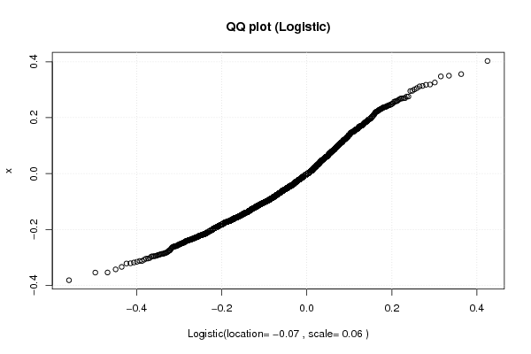
xlab <- paste('Logistic(location=',round(f$estimate[[1]],2))
xlab <- paste(xlab,', scale=')
xlab <- paste(xlab,round(f$estimate[[2]],2))
xlab <- paste(xlab,')')
bitmap(file='test2.png')
qqplot(qlogis(ppoints(x), location=f$estimate[[1]], scale=f$estimate[[2]]), x, main='QQ plot (Logistic)', xlab=xlab )
grid()
dev.off()
load(file='createtable')
a<-table.start()
a<-table.row.start(a)
a<-table.element(a,'Parameter',1,TRUE)
a<-table.element(a,'Estimated Value',1,TRUE)
a<-table.element(a,'Standard Deviation',1,TRUE)
a<-table.row.end(a)
a<-table.row.start(a)
a<-table.element(a,'location',header=TRUE)
a<-table.element(a,f$estimate[1])
a<-table.element(a,f$sd[1])
a<-table.row.end(a)
a<-table.row.start(a)
a<-table.element(a,'scale',header=TRUE)
a<-table.element(a,f$estimate[2])
a<-table.element(a,f$sd[2])
a<-table.row.end(a)
a<-table.end(a)
table.save(a,file='mytable.tab')