Repository of Reproducible Computations

Free Statistics

of Irreproducible Research!

Author's title

Author

*The author of this computation has been verified*

R Software Module

rwasp_boxcoxnorm.wasp

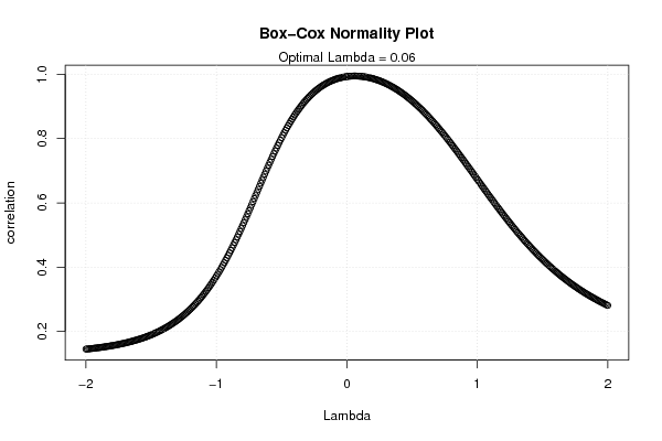
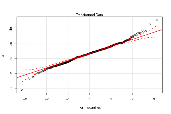
Title produced by software

Box-Cox Normality Plot

Date of computation

Thu, 21 Dec 2017 22:03:12 +0100

Cite this page as follows

Statistical Computations at FreeStatistics.org, Office for Research Development and Education, URL https://freestatistics.org/blog/index.php?v=date/2017/Dec/21/t1513890232p3vt2y39wvgb49a.htm/, Retrieved Tue, 14 May 2024 20:45:16 +0000

Statistical Computations at FreeStatistics.org, Office for Research Development and Education, URL https://freestatistics.org/blog/index.php?pk=310733, Retrieved Tue, 14 May 2024 20:45:16 +0000

QR Codes:

Paste this QR Code to cite your computation.

Original text written by user:

IsPrivate?

No (this computation is public)

User-defined keywords

Estimated Impact

Family? (F = Feedback message, R = changed R code, M = changed R Module, P = changed Parameters, D = changed Data)

-       [Box-Cox Normality Plot] [Box-Cox Normality...] [2017-12-21 21:03:12] [f7fcbef48f036f8c57e773abb9891403] [Current]

Feedback Forum

Post a new message

Dataseries X:

Download CSV

Histogram

Boxplots

83674204.92
1780582985.50
75198229.43
66552858.02
47377292.82
202450191.48
139917216.59
129019740.35
70169361.12
49375016.78
59073785.95
89062635.98
149805035.68
121657356.12
53218003.32
134314180.33
41501724.73
101190684.88
78601349.78
41458023.49
124456725.54
175844207.75
95041211.77
47068781.84
60350058.62
85555510.86
64400011.97
116681743.38
88648506.56
69194523.37
51115705.16
100175600.31
111989704.69
87312371.62
189344006.44
164413751.73
389423515.99
102126834.31
82120289.65
90980789.21
41278167.54
108959432.50
110751384.31
45096581.99
5530000.01
91412977.98
82847784.50
36612438.99
181071513.72
53746879.90
124559250.64
36698020.15
62934778.95
73414447.19
45884687.67
87832898.47
73069485.61
42195466.42
35830154.17
156770436.11
54294999.18
58513045.36
43527242.04
43205602.28
44706884.64
160914168.27
35082993.05
59822334.79
112211208.73
65205148.09
238077836.32
165219181.12
86130405.49
461964651.71
171139517.93
111032333.28
180249086.05
77894859.75
356473658.26
166542522.62
54125197.52
168151470.10
135764498.43
37570670.97
315804194.31
423707340.96
135714858.80
243733834.55
237163226.09
161036493.87
143348790.49
10888021.53
237468586.59
46198566.04
51437155.59
209130115.72
176879819.50
35045038.21
65096793.73
73508446.84
51708403.59
58292306.49
102123580.00
53158301.57
124494225.89
91583660.26
76281205.42
163529644.28
26774034.54
144704279.83
69114646.47
86950644.80
175990756.79
158929908.10
148155746.78
62779862.12
19818260.44
88601705.01
30007930.38
117832980.18
90848930.71
89397843.03
55263706.65
69991137.65
143797027.39
52673003.03
28706022.10
62998324.49
67833116.68
75723475.10
48325193.00
111360028.58
24660326.90
82460584.67
145281782.55
39486520.21
60947767.64
60121930.24
99017214.81
35238165.30
123420536.16
74746463.17
562343449.26
94683693.97
81904382.19
99095998.96
142175940.20
155903769.11
78634994.57
36977845.61
34414962.16
102341645.98
56237645.75
27172686.96
41273198.60
216175606.08
55898647.10
75221385.94
53676891.83
81091784.87
77042398.81
28174938.67
35101461.83
68538574.63
44615475.28
43069115.58
143983064.34
46825971.36
134566048.14
90240422.37
56049938.72
175425686.55
176518866.51
40669236.13
15735297.80
98139206.91
41803620.00
158877910.97
30399756.30
47388802.69
41728417.19
69231928.02
71853610.07
558959084.34
52566146.36
71674599.90
110358574.86
84597608.62
101107225.10
13370105.37
194211934.95
57318082.47
32536505.48
30275241.72
43088560.58
10752495.01
134197141.73
2050754.56
65419855.94
61175707.93
45614657.12
23662737.25
27092741.28
11126014.61
65593377.32
37809417.15
50054204.29
110486000.24
325943399.04
49870777.29
23695745.49
108184247.16
164542311.66
125549650.35
107449263.65
8393570.83
72757794.21
48819423.37
50421429.43
68645643.01
263997474.96
37709829.83
58817989.39
41975398.72
41109010.86
108335047.35
34635284.88
34146816.44
40027824.91
255413911.10
39327036.60
34338165.77
40263957.24
29123563.03
25270133.49
21427131.27
83583036.21
37173439.19
55380715.77
33827105.84
15154155.13
37461595.38
127294245.12
43078336.44
42758206.49
383900334.78
87822482.33
141180713.72
90298133.84
86505418.31
90694450.78
167910891.25
50607613.62
135425474.89
102720180.37
66857581.76
73816862.43
207318845.32
99802773.49
67851606.53
86801450.06
61288989.68
113177815.47
54967014.24
81001444.77
62918316.25
79742451.05
29333512.89
94972892.77
26549874.17
47579300.90
105920074.84
150747468.10
77872467.76
105931079.33
167937296.54
67982977.64
1127522650.64
33917970.01
122322917.57
51191129.67
62534355.27
147382680.51
29776722.78
62470751.06
62340306.49
76224265.73
70626921.41
34032560.79
34234210.43
38939478.00
70303064.10
42727099.37
147403937.87
76803541.00
35977424.43
66205410.90
28025110.03
33531833.06
10151610.61
31918395.56
31383005.56
42887668.11
236404571.67
78960632.59
175788801.46
91832230.46
306046912.37
78331944.89
131983592.11
120919736.51
48935304.19
38373571.39
13482490.40
26820678.58
24159621.41
15019293.19
44094415.15
43221355.88
472963673.61
84489770.96
92558087.82
19273066.83
71065080.27
53076402.93
63601168.39
62866732.28
52874069.45
77463960.29
51942683.95
34252330.78
48107684.67
48876597.95
47073139.89
64901297.63
20289119.53
55054846.84
17940235.70
334072416.20
44388206.89
18310249.52
83896494.88
45722559.76
21836599.30
35118855.23
150765293.54
42201875.01
92723742.48
64474835.50
216962470.14
64400374.43
37629453.81
41434942.09
107382240.34
43023288.68
33909234.14
24467489.05
103834428.13
28659746.45
27671595.46
10962990.77
25238585.05
14135312.91
12952681.63
63439160.04
30006711.39
76152933.75
57222458.69
15673507.41
23649020.47
20416603.84
29797853.38
18958200.07
52901004.30
17401244.28
247393964.80
27080730.38
50451316.51
14470807.48
50823410.95
16614593.12
19358791.49
20497331.08
14199402.87
24633296.00
77518810.76
23520963.94
19995502.56
36034129.65
11122663.82
21201785.37
30503260.49
60550877.27
20320083.81
18597081.06
13308985.77
97603695.92
41843004.31
47124618.11
34820600.19
40156382.31
124578471.31
18582757.50
34038496.74
71144154.14
58098157.86
106321597.38
41691766.42
610101644.52
90944470.74
55309626.74
166135384.26
67216592.50
72174542.68
65801713.92
64816227.13
62085580.91
83483908.03
62917735.31
34295119.05
13574588.68
17416253.17
17727082.01
13431085.51
15172534.44
32540943.64
68775834.47
75444608.45
40462339.40
20772249.10
12345912.81
20373311.51
16455535.66
41430238.43
22237504.51
34029916.05
21232392.13
25249850.80
37982401.65
25217298.61
13068829.57
54488407.77
153120189.19
22855597.19
36810206.96
8419073.01
5730916.51
27858675.43
26261553.11
14590398.03
29541770.29
16371957.79
16291258.87
15857207.06
17038776.18
74697561.03
15452944.58
16912129.43
29259761.68
25248097.12
65919010.85
12207281.77
20251395.73
33416732.62
159605911.86
85079503.42
210834140.85
37364693.10
40564843.01
373521155.87
56683585.68
55883410.76
65487353.48
27817774.15
39922107.66
166458725.96
82156772.62
92996093.99
30743914.40
43275684.47
118542707.01
40563761.39
55855949.38
33426012.30
115874023.29
83855415.36
56925213.51
51740733.34
61084521.87
36774358.09
44711837.49
98317957.16
47860971.78
64488518.70
53036656.78
126762831.05
43174170.46
27015027.09
377094.66
39780669.38
38430137.95
79391438.56
55962069.52
123858678.91
30871857.27
101837566.51
12492775.95
60644882.76
10761253.54
19468295.42
2581083.89
12003062.33
33355567.04
8548450.87
4352375.82
14097650.14
22182800.06
12568081.02
10751225.95
6192572.47
36480577.72
10643018.21
17256072.97
11217260.51
60230572.58
18626805.04
8143091.44
8868805.11
12081820.83
24543956.74
15324447.45
4029081.46
4508075.47
11215550.35
16978476.17
19877893.21
15024577.84
17849749.24
8642730.53
9848011.81
36834521.18
13620030.75
12365667.12
15223219.31
7789669.15
7466085.12
6976990.54
10294001.25
29128119.83
17566176.81
5291185.49
25925453.45
27495855.35
9232653.29
60779131.03
44433224.98
13931267.71
30661156.64
18623146.14
16539661.47
11536267.35
42275408.79
19488550.80
41853937.29
14800207.11
6850020.18
93057221.42
35630707.07
78547195.23
36872176.19
41340222.51
35522149.25
53223208.40
476285852.47
19876445.65
58674083.89
36952141.39
90502312.85
39352343.78
71925661.24
51024382.09
129304683.64
16456921.89
38822191.84
8658219.76
39750993.31
30368830.19
76371351.34
15554523.77

Summary of computational transaction
Raw Input	view raw input (R code)
Raw Output	view raw output of R engine
Computing time	5 seconds
R Server	Big Analytics Cloud Computing Center

\begin{tabular}{lllllllll}
\hline
Summary of computational transaction \tabularnewline
Raw Input view raw input (R code)  \tabularnewline
Raw Outputview raw output of R engine  \tabularnewline
Computing time5 seconds \tabularnewline
R ServerBig Analytics Cloud Computing Center \tabularnewline
\hline
\end{tabular}
%Source: https://freestatistics.org/blog/index.php?pk=310733&T=0

[TABLE]
[ROW]

Summary of computational transaction[/C][/ROW] [ROW]

Raw Input[/C]

view raw input (R code) [/C][/ROW] [ROW]

Raw Output[/C]

view raw output of R engine [/C][/ROW] [ROW]

Computing time[/C]

5 seconds[/C][/ROW] [ROW]

R Server[/C]

Big Analytics Cloud Computing Center[/C][/ROW] [/TABLE] Source: https://freestatistics.org/blog/index.php?pk=310733&T=0

Globally Unique Identifier (entire table): ba.freestatistics.org/blog/index.php?pk=310733&T=0

As an alternative you can also use a QR Code:

The GUIDs for individual cells are displayed in the table below:

Summary of computational transaction
Raw Input	view raw input (R code)
Raw Output	view raw output of R engine
Computing time	5 seconds
R Server	Big Analytics Cloud Computing Center

Box-Cox Normality Plot
# observations x	589
maximum correlation	0.994239038632349
optimal lambda	0.06
transformation formula	for all lambda <> 0 : T(Y) = (Y^lambda - 1) / lambda

\begin{tabular}{lllllllll}
\hline
Box-Cox Normality Plot \tabularnewline
# observations x & 589 \tabularnewline
maximum correlation & 0.994239038632349 \tabularnewline
optimal lambda & 0.06 \tabularnewline
transformation formula & for all lambda <> 0 : T(Y) = (Y^lambda - 1) / lambda \tabularnewline
\hline
\end{tabular}
%Source: https://freestatistics.org/blog/index.php?pk=310733&T=1

[TABLE]
[ROW][C]Box-Cox Normality Plot[/C][/ROW]
[ROW][C]# observations x[/C][C]589[/C][/ROW]
[ROW][C]maximum correlation[/C][C]0.994239038632349[/C][/ROW]
[ROW][C]optimal lambda[/C][C]0.06[/C][/ROW]
[ROW][C]transformation formula[/C][C]for all lambda <> 0 : T(Y) = (Y^lambda - 1) / lambda[/C][/ROW]
[/TABLE]
Source: https://freestatistics.org/blog/index.php?pk=310733&T=1

Globally Unique Identifier (entire table): ba.freestatistics.org/blog/index.php?pk=310733&T=1

As an alternative you can also use a QR Code:

The GUIDs for individual cells are displayed in the table below:

Box-Cox Normality Plot
# observations x	589
maximum correlation	0.994239038632349
optimal lambda	0.06
transformation formula	for all lambda <> 0 : T(Y) = (Y^lambda - 1) / lambda

Maximum Likelihood Estimation of Lambda

> summary(mypT)
bcPower Transformation to Normality 
  Est Power Rounded Pwr Wald Lwr bnd Wald Upr Bnd
x    0.0597        0.06       0.0023       0.1171
Likelihood ratio tests about transformation parameters
                              LRT df       pval
LR test, lambda = (0)    4.222829  1 0.03988361
LR test, lambda = (1) 1032.519290  1 0.00000000

\begin{tabular}{lllllllll}
\hline
Maximum Likelihood Estimation of Lambda \tabularnewline
> summary(mypT)
bcPower Transformation to Normality 
  Est Power Rounded Pwr Wald Lwr bnd Wald Upr Bnd
x    0.0597        0.06       0.0023       0.1171
Likelihood ratio tests about transformation parameters
                              LRT df       pval
LR test, lambda = (0)    4.222829  1 0.03988361
LR test, lambda = (1) 1032.519290  1 0.00000000
 \tabularnewline
\hline
\end{tabular}
%Source: https://freestatistics.org/blog/index.php?pk=310733&T=2

[TABLE]
[ROW][C]Maximum Likelihood Estimation of Lambda[/C][/ROW]
[ROW][C]> summary(mypT)
bcPower Transformation to Normality 
  Est Power Rounded Pwr Wald Lwr bnd Wald Upr Bnd
x    0.0597        0.06       0.0023       0.1171
Likelihood ratio tests about transformation parameters
                              LRT df       pval
LR test, lambda = (0)    4.222829  1 0.03988361
LR test, lambda = (1) 1032.519290  1 0.00000000
[/C][/ROW]
[/TABLE]
Source: https://freestatistics.org/blog/index.php?pk=310733&T=2

Globally Unique Identifier (entire table): ba.freestatistics.org/blog/index.php?pk=310733&T=2

As an alternative you can also use a QR Code:

The GUIDs for individual cells are displayed in the table below:

Maximum Likelihood Estimation of Lambda

> summary(mypT)
bcPower Transformation to Normality 
  Est Power Rounded Pwr Wald Lwr bnd Wald Upr Bnd
x    0.0597        0.06       0.0023       0.1171
Likelihood ratio tests about transformation parameters
                              LRT df       pval
LR test, lambda = (0)    4.222829  1 0.03988361
LR test, lambda = (1) 1032.519290  1 0.00000000

Figure 1

PNG link

Postscript link

PDF link

Figure 2

PNG link

Postscript link

PDF link

Figure 3

PNG link

Postscript link

PDF link

Figure 4

PNG link

Postscript link

PDF link

Figure 5

PNG link

Postscript link

PDF link

Parameters (Session):

par1 = Full Box-Cox transform ; par2 = -2 ; par3 = 2 ; par4 = 0 ; par5 = No ;

Parameters (R input):

par1 = Full Box-Cox transform ; par2 = -2 ; par3 = 2 ; par4 = 0 ; par5 = No ;

R code (references can be found in the software module):

library(car)
par2 <- abs(as.numeric(par2)*100)
par3 <- as.numeric(par3)*100
if(par4=='') par4 <- 0
par4 <- as.numeric(par4)
numlam <- par2 + par3 + 1
x <- x + par4
n <- length(x)
c <- array(NA,dim=c(numlam))
l <- array(NA,dim=c(numlam))
mx <- -1
mxli <- -999
for (i in 1:numlam)
{
l[i] <- (i-par2-1)/100
if (l[i] != 0)
{
if (par1 == 'Full Box-Cox transform') x1 <- (x^l[i] - 1) / l[i]
if (par1 == 'Simple Box-Cox transform') x1 <- x^l[i]
} else {
x1 <- log(x)
}
c[i] <- cor(qnorm(ppoints(x), mean=0, sd=1),sort(x1))
if (mx < c[i])
{
mx <- c[i]
mxli <- l[i]
x1.best <- x1
}
}
print(c)
print(mx)
print(mxli)
print(x1.best)
if (mxli != 0)
{
if (par1 == 'Full Box-Cox transform') x1 <- (x^mxli - 1) / mxli
if (par1 == 'Simple Box-Cox transform') x1 <- x^mxli
} else {
x1 <- log(x)
}
mypT <- powerTransform(x)
summary(mypT)
bitmap(file='test1.png')
plot(l,c,main='Box-Cox Normality Plot', xlab='Lambda',ylab='correlation')
mtext(paste('Optimal Lambda =',mxli))
grid()
dev.off()
bitmap(file='test2.png')
hist(x,main='Histogram of Original Data',xlab='X',ylab='frequency')
grid()
dev.off()
bitmap(file='test3.png')
hist(x1,main='Histogram of Transformed Data', xlab='X',ylab='frequency')
grid()
dev.off()
bitmap(file='test4.png')
qqPlot(x)
grid()
mtext('Original Data')
dev.off()
bitmap(file='test5.png')
qqPlot(x1)
grid()
mtext('Transformed Data')
dev.off()
load(file='createtable')
a<-table.start()
a<-table.row.start(a)
a<-table.element(a,'Box-Cox Normality Plot',2,TRUE)
a<-table.row.end(a)
a<-table.row.start(a)
a<-table.element(a,'# observations x',header=TRUE)
a<-table.element(a,n)
a<-table.row.end(a)
a<-table.row.start(a)
a<-table.element(a,'maximum correlation',header=TRUE)
a<-table.element(a,mx)
a<-table.row.end(a)
a<-table.row.start(a)
a<-table.element(a,'optimal lambda',header=TRUE)
a<-table.element(a,mxli)
a<-table.row.end(a)
a<-table.row.start(a)
a<-table.element(a,'transformation formula',header=TRUE)
if (par1 == 'Full Box-Cox transform') {
a<-table.element(a,'for all lambda <> 0 : T(Y) = (Y^lambda - 1) / lambda')
} else {
a<-table.element(a,'for all lambda <> 0 : T(Y) = Y^lambda')
}
a<-table.row.end(a)
if(mx<0) {
a<-table.row.start(a)
a<-table.element(a,'Warning: maximum correlation is negative! The Box-Cox transformation must not be used.',2)
a<-table.row.end(a)
}
a<-table.end(a)
table.save(a,file='mytable.tab')
if(par5=='Yes') {
a<-table.start()
a<-table.row.start(a)
a<-table.element(a,'Obs.',header=T)
a<-table.element(a,'Original',header=T)
a<-table.element(a,'Transformed',header=T)
a<-table.row.end(a)
for (i in 1:n) {
a<-table.row.start(a)
a<-table.element(a,i)
a<-table.element(a,x[i])
a<-table.element(a,x1.best[i])
a<-table.row.end(a)
}
a<-table.end(a)
table.save(a,file='mytable1.tab')
}
a<-table.start()
a<-table.row.start(a)
a<-table.element(a,'Maximum Likelihood Estimation of Lambda',1,TRUE)
a<-table.row.end(a)
a<-table.row.start(a)
a<-table.element(a,paste('',RC.texteval('summary(mypT)'),'
',sep=''))
a<-table.row.end(a)
a<-table.end(a)
table.save(a,file='mytable3.tab')

Free Statistics

Description of Statistical Computation

Tree of Dependent Computations

Dataset

Tables (Output of Computation)

Figures (Output of Computation)

Input Parameters & R Code