Free Statistics
of Irreproducible Research!
Description of Statistical Computation | ||||||||||||||||||||||||||||||||||||||||||||||||
|---|---|---|---|---|---|---|---|---|---|---|---|---|---|---|---|---|---|---|---|---|---|---|---|---|---|---|---|---|---|---|---|---|---|---|---|---|---|---|---|---|---|---|---|---|---|---|---|---|
| Author's title | ||||||||||||||||||||||||||||||||||||||||||||||||
| Author | *The author of this computation has been verified* | |||||||||||||||||||||||||||||||||||||||||||||||
| R Software Module | rwasp_fitdistrnorm.wasp | |||||||||||||||||||||||||||||||||||||||||||||||
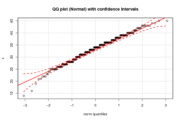
| Title produced by software | ML Fitting and QQ Plot- Normal Distribution | |||||||||||||||||||||||||||||||||||||||||||||||
| Date of computation | Tue, 19 Dec 2017 11:44:43 +0100 | |||||||||||||||||||||||||||||||||||||||||||||||
| Cite this page as follows | Statistical Computations at FreeStatistics.org, Office for Research Development and Education, URL https://freestatistics.org/blog/index.php?v=date/2017/Dec/19/t1513681004nu8anj7dnegp1n1.htm/, Retrieved Thu, 16 May 2024 02:23:03 +0000 | |||||||||||||||||||||||||||||||||||||||||||||||
| Statistical Computations at FreeStatistics.org, Office for Research Development and Education, URL https://freestatistics.org/blog/index.php?pk=310274, Retrieved Thu, 16 May 2024 02:23:03 +0000 | ||||||||||||||||||||||||||||||||||||||||||||||||
| QR Codes: | ||||||||||||||||||||||||||||||||||||||||||||||||
|
| ||||||||||||||||||||||||||||||||||||||||||||||||
| Original text written by user: | ||||||||||||||||||||||||||||||||||||||||||||||||
| IsPrivate? | No (this computation is public) | |||||||||||||||||||||||||||||||||||||||||||||||
| User-defined keywords | ||||||||||||||||||||||||||||||||||||||||||||||||
| Estimated Impact | 113 | |||||||||||||||||||||||||||||||||||||||||||||||
Tree of Dependent Computations | ||||||||||||||||||||||||||||||||||||||||||||||||
| Family? (F = Feedback message, R = changed R code, M = changed R Module, P = changed Parameters, D = changed Data) | ||||||||||||||||||||||||||||||||||||||||||||||||
| - [ML Fitting and QQ Plot- Normal Distribution] [normal QQ-plot] [2017-12-19 10:44:43] [265bf64618ae5fabb4f8135a65428bee] [Current] | ||||||||||||||||||||||||||||||||||||||||||||||||
| Feedback Forum | ||||||||||||||||||||||||||||||||||||||||||||||||
Post a new message | ||||||||||||||||||||||||||||||||||||||||||||||||
Dataset | ||||||||||||||||||||||||||||||||||||||||||||||||
| Dataseries X: | ||||||||||||||||||||||||||||||||||||||||||||||||
22 39 40 34 38 39 39 38 31 34 32 37 36 38 29 33 35 34 45 30 33 30 40 34 31 27 33 42 36 33 42 33 21 43 34 32 34 28 30 27 29 40 29 41 33 42 39 35 33 33 44 34 30 30 35 39 34 39 25 39 33 34 36 34 31 35 34 36 40 31 33 28 42 38 35 34 28 35 25 39 25 32 35 41 34 33 32 34 25 38 37 38 36 39 31 40 34 33 32 33 32 28 32 34 36 38 31 36 27 31 28 30 29 29 31 35 42 28 38 34 28 30 26 27 31 35 33 34 30 28 30 29 32 34 34 35 40 34 28 35 31 33 36 30 27 30 25 39 36 31 33 30 31 32 33 43 35 36 42 31 26 38 27 27 31 32 36 36 25 33 32 40 36 36 35 31 31 36 36 37 31 31 26 35 32 36 37 34 33 35 31 38 36 32 28 33 31 34 33 36 36 29 31 35 31 35 36 35 38 28 28 28 34 31 44 36 36 34 32 36 38 28 37 32 36 30 38 37 33 43 26 33 34 36 36 36 36 39 33 35 25 26 35 16 40 14 22 21 38 38 27 40 40 19 29 37 27 26 24 29 26 27 35 39 38 36 37 36 32 33 39 34 39 36 33 30 39 37 37 35 32 36 36 41 36 37 29 39 37 32 36 43 30 33 28 30 28 39 34 34 29 32 33 27 35 38 40 34 34 26 39 34 39 26 30 34 34 29 41 43 31 33 34 30 23 29 35 40 27 30 27 29 33 32 33 36 34 45 30 22 24 25 26 27 27 35 36 32 35 35 36 37 33 25 35 37 36 35 29 35 31 30 37 36 35 32 34 37 36 39 37 31 40 38 35 38 32 41 28 40 25 28 37 37 40 26 30 32 31 28 34 39 33 43 37 31 31 34 32 27 34 28 32 39 28 39 32 36 31 39 23 25 32 32 36 39 31 32 28 34 28 38 35 32 26 32 28 31 33 38 38 36 31 36 43 37 28 35 34 40 31 41 35 38 37 31 | ||||||||||||||||||||||||||||||||||||||||||||||||
Tables (Output of Computation) | ||||||||||||||||||||||||||||||||||||||||||||||||
| ||||||||||||||||||||||||||||||||||||||||||||||||
Figures (Output of Computation) | ||||||||||||||||||||||||||||||||||||||||||||||||
Input Parameters & R Code | ||||||||||||||||||||||||||||||||||||||||||||||||
| Parameters (Session): | ||||||||||||||||||||||||||||||||||||||||||||||||
| par1 = 8 ; par2 = 0 ; | ||||||||||||||||||||||||||||||||||||||||||||||||
| Parameters (R input): | ||||||||||||||||||||||||||||||||||||||||||||||||
| par1 = 8 ; par2 = 0 ; | ||||||||||||||||||||||||||||||||||||||||||||||||
| R code (references can be found in the software module): | ||||||||||||||||||||||||||||||||||||||||||||||||
library(MASS) | ||||||||||||||||||||||||||||||||||||||||||||||||