Free Statistics
of Irreproducible Research!
Description of Statistical Computation | ||||||||||||||||||||||||||||||||||||||||||||||||||||||
|---|---|---|---|---|---|---|---|---|---|---|---|---|---|---|---|---|---|---|---|---|---|---|---|---|---|---|---|---|---|---|---|---|---|---|---|---|---|---|---|---|---|---|---|---|---|---|---|---|---|---|---|---|---|---|
| Author's title | ||||||||||||||||||||||||||||||||||||||||||||||||||||||
| Author | *The author of this computation has been verified* | |||||||||||||||||||||||||||||||||||||||||||||||||||||
| R Software Module | rwasp_bidensity.wasp | |||||||||||||||||||||||||||||||||||||||||||||||||||||
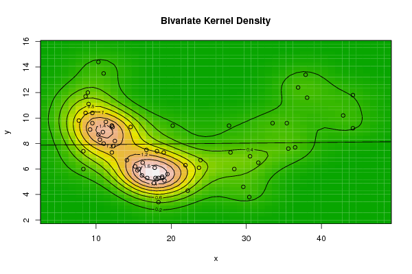
| Title produced by software | Bivariate Kernel Density Estimation | |||||||||||||||||||||||||||||||||||||||||||||||||||||
| Date of computation | Mon, 18 Dec 2017 15:03:37 +0100 | |||||||||||||||||||||||||||||||||||||||||||||||||||||
| Cite this page as follows | Statistical Computations at FreeStatistics.org, Office for Research Development and Education, URL https://freestatistics.org/blog/index.php?v=date/2017/Dec/18/t1513605883f6bd866mlo89sjw.htm/, Retrieved Tue, 14 May 2024 18:08:36 +0000 | |||||||||||||||||||||||||||||||||||||||||||||||||||||
| Statistical Computations at FreeStatistics.org, Office for Research Development and Education, URL https://freestatistics.org/blog/index.php?pk=310184, Retrieved Tue, 14 May 2024 18:08:36 +0000 | ||||||||||||||||||||||||||||||||||||||||||||||||||||||
| QR Codes: | ||||||||||||||||||||||||||||||||||||||||||||||||||||||
|
| ||||||||||||||||||||||||||||||||||||||||||||||||||||||
| Original text written by user: | ||||||||||||||||||||||||||||||||||||||||||||||||||||||
| IsPrivate? | No (this computation is public) | |||||||||||||||||||||||||||||||||||||||||||||||||||||
| User-defined keywords | ||||||||||||||||||||||||||||||||||||||||||||||||||||||
| Estimated Impact | 58 | |||||||||||||||||||||||||||||||||||||||||||||||||||||
Tree of Dependent Computations | ||||||||||||||||||||||||||||||||||||||||||||||||||||||
| Family? (F = Feedback message, R = changed R code, M = changed R Module, P = changed Parameters, D = changed Data) | ||||||||||||||||||||||||||||||||||||||||||||||||||||||
| - [Bivariate Kernel Density Estimation] [] [2017-12-18 14:03:37] [f1ade19563a25eb31edff11eb9af1158] [Current] | ||||||||||||||||||||||||||||||||||||||||||||||||||||||
| Feedback Forum | ||||||||||||||||||||||||||||||||||||||||||||||||||||||
Post a new message | ||||||||||||||||||||||||||||||||||||||||||||||||||||||
Dataset | ||||||||||||||||||||||||||||||||||||||||||||||||||||||
| Dataseries X: | ||||||||||||||||||||||||||||||||||||||||||||||||||||||
37,90 22,20 44,20 16,70 12,10 9,50 18,80 11,30 14,10 35,40 10,30 12,30 16,10 33,50 29,60 36,50 12,20 8,60 30,50 19,00 16,20 17,90 30,40 18,10 8,60 27,70 7,70 23,90 31,60 19,10 18,30 17,70 38,10 18,10 19,50 10,90 44,20 36,90 14,60 21,90 17,80 23,70 9,50 9,00 8,90 11,00 18,30 20,20 8,30 9,20 15,20 27,90 12,10 10,50 8,30 35,60 11,00 15,70 42,90 10,30 12,10 12,50 16,80 18,80 15,50 28,40 | ||||||||||||||||||||||||||||||||||||||||||||||||||||||
| Dataseries Y: | ||||||||||||||||||||||||||||||||||||||||||||||||||||||
13,40 4,30 9,20 7,50 7,30 9,60 5,40 9,70 6,70 9,60 8,70 7,80 5,50 9,60 4,60 7,70 9,30 11,70 7,00 7,30 6,50 5,30 3,80 5,20 10,40 9,40 9,80 6,70 6,50 5,10 5,30 4,90 11,60 7,40 5,60 8,90 11,80 12,40 9,30 6,30 6,10 6,10 10,40 11,10 12,00 13,50 3,40 9,40 6,00 9,10 6,20 7,30 9,40 8,30 7,40 7,60 8,00 6,00 10,20 14,40 9,40 8,20 5,30 5,30 5,90 6,00 | ||||||||||||||||||||||||||||||||||||||||||||||||||||||
Tables (Output of Computation) | ||||||||||||||||||||||||||||||||||||||||||||||||||||||
| ||||||||||||||||||||||||||||||||||||||||||||||||||||||
Figures (Output of Computation) | ||||||||||||||||||||||||||||||||||||||||||||||||||||||
Input Parameters & R Code | ||||||||||||||||||||||||||||||||||||||||||||||||||||||
| Parameters (Session): | ||||||||||||||||||||||||||||||||||||||||||||||||||||||
| par1 = 50 ; par2 = 50 ; par3 = 0 ; par4 = 0 ; par5 = 0 ; par6 = Y ; par7 = Y ; par8 = terrain.colors ; | ||||||||||||||||||||||||||||||||||||||||||||||||||||||
| Parameters (R input): | ||||||||||||||||||||||||||||||||||||||||||||||||||||||
| par1 = 50 ; par2 = 50 ; par3 = 0 ; par4 = 0 ; par5 = 0 ; par6 = Y ; par7 = Y ; par8 = terrain.colors ; | ||||||||||||||||||||||||||||||||||||||||||||||||||||||
| R code (references can be found in the software module): | ||||||||||||||||||||||||||||||||||||||||||||||||||||||
par1 <- as(par1,'numeric') | ||||||||||||||||||||||||||||||||||||||||||||||||||||||