Free Statistics
of Irreproducible Research!
Description of Statistical Computation | ||||||||||||||||||||||||||||||||||||||||||||||||||||||||||
|---|---|---|---|---|---|---|---|---|---|---|---|---|---|---|---|---|---|---|---|---|---|---|---|---|---|---|---|---|---|---|---|---|---|---|---|---|---|---|---|---|---|---|---|---|---|---|---|---|---|---|---|---|---|---|---|---|---|---|
| Author's title | ||||||||||||||||||||||||||||||||||||||||||||||||||||||||||
| Author | *The author of this computation has been verified* | |||||||||||||||||||||||||||||||||||||||||||||||||||||||||
| R Software Module | rwasp_tukeylambda.wasp | |||||||||||||||||||||||||||||||||||||||||||||||||||||||||
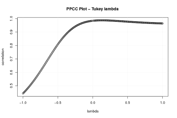
| Title produced by software | Tukey lambda PPCC Plot | |||||||||||||||||||||||||||||||||||||||||||||||||||||||||
| Date of computation | Mon, 18 Dec 2017 09:18:35 +0100 | |||||||||||||||||||||||||||||||||||||||||||||||||||||||||
| Cite this page as follows | Statistical Computations at FreeStatistics.org, Office for Research Development and Education, URL https://freestatistics.org/blog/index.php?v=date/2017/Dec/18/t15135851374oj051pplpjm7g7.htm/, Retrieved Tue, 14 May 2024 02:49:54 +0000 | |||||||||||||||||||||||||||||||||||||||||||||||||||||||||
| Statistical Computations at FreeStatistics.org, Office for Research Development and Education, URL https://freestatistics.org/blog/index.php?pk=310087, Retrieved Tue, 14 May 2024 02:49:54 +0000 | ||||||||||||||||||||||||||||||||||||||||||||||||||||||||||
| QR Codes: | ||||||||||||||||||||||||||||||||||||||||||||||||||||||||||
|
| ||||||||||||||||||||||||||||||||||||||||||||||||||||||||||
| Original text written by user: | ||||||||||||||||||||||||||||||||||||||||||||||||||||||||||
| IsPrivate? | No (this computation is public) | |||||||||||||||||||||||||||||||||||||||||||||||||||||||||
| User-defined keywords | ||||||||||||||||||||||||||||||||||||||||||||||||||||||||||
| Estimated Impact | 90 | |||||||||||||||||||||||||||||||||||||||||||||||||||||||||
Tree of Dependent Computations | ||||||||||||||||||||||||||||||||||||||||||||||||||||||||||
| Family? (F = Feedback message, R = changed R code, M = changed R Module, P = changed Parameters, D = changed Data) | ||||||||||||||||||||||||||||||||||||||||||||||||||||||||||
| - [Tukey lambda PPCC Plot] [] [2017-12-18 08:18:35] [de41148bc22dc60de494a82836f9abe5] [Current] | ||||||||||||||||||||||||||||||||||||||||||||||||||||||||||
| Feedback Forum | ||||||||||||||||||||||||||||||||||||||||||||||||||||||||||
Post a new message | ||||||||||||||||||||||||||||||||||||||||||||||||||||||||||
Dataset | ||||||||||||||||||||||||||||||||||||||||||||||||||||||||||
| Dataseries X: | ||||||||||||||||||||||||||||||||||||||||||||||||||||||||||
14 21 20 20 20 18 18 17 15 18 16 17 19 21 15 21 16 18 18 17 18 16 15 15 19 14 19 19 15 17 21 13 12 15 19 19 14 18 11 17 18 13 12 17 20 16 22 16 23 20 23 13 18 18 17 17 18 21 13 19 16 17 18 18 12 19 16 20 21 18 13 17 20 21 19 15 14 15 16 19 17 17 15 19 21 19 18 18 15 19 19 18 20 18 12 15 17 15 17 20 11 14 14 12 19 22 16 15 15 18 12 17 10 10 18 16 22 12 10 20 20 19 10 13 15 19 17 15 12 14 13 15 20 12 16 15 17 15 12 17 11 16 16 15 17 7 14 21 20 15 13 20 15 16 19 16 19 17 19 14 16 16 14 11 17 20 20 17 13 20 17 16 19 20 17 14 20 19 18 17 17 10 12 19 19 21 21 17 19 21 15 14 15 13 14 14 19 17 19 18 21 12 15 19 16 19 16 18 18 15 15 11 18 13 9 21 19 13 15 18 16 10 12 18 17 15 16 19 15 24 15 14 16 16 20 20 20 20 14 22 16 9 14 11 23 10 10 8 21 18 15 20 17 5 14 19 15 12 10 11 15 15 20 20 20 19 16 21 22 17 21 19 23 21 22 11 20 18 16 18 13 17 20 20 15 18 15 19 19 19 20 20 16 18 17 18 13 20 21 17 19 20 15 15 19 18 22 20 18 14 15 17 16 17 15 17 18 16 18 22 16 16 20 18 16 16 20 21 18 15 18 18 20 18 16 19 20 22 18 8 13 13 18 12 16 21 20 18 22 23 23 21 16 14 18 22 20 18 12 17 15 18 18 15 16 15 16 19 19 23 20 18 21 19 18 19 17 21 19 24 12 15 18 19 22 19 16 19 18 18 19 21 19 22 23 17 18 19 15 14 18 17 19 16 14 20 16 18 16 21 16 14 16 19 19 19 18 16 14 19 11 18 18 16 20 18 20 16 18 19 19 15 17 21 24 16 13 21 16 17 17 18 18 23 20 20 | ||||||||||||||||||||||||||||||||||||||||||||||||||||||||||
Tables (Output of Computation) | ||||||||||||||||||||||||||||||||||||||||||||||||||||||||||
| ||||||||||||||||||||||||||||||||||||||||||||||||||||||||||
Figures (Output of Computation) | ||||||||||||||||||||||||||||||||||||||||||||||||||||||||||
Input Parameters & R Code | ||||||||||||||||||||||||||||||||||||||||||||||||||||||||||
| Parameters (Session): | ||||||||||||||||||||||||||||||||||||||||||||||||||||||||||
| Parameters (R input): | ||||||||||||||||||||||||||||||||||||||||||||||||||||||||||
| R code (references can be found in the software module): | ||||||||||||||||||||||||||||||||||||||||||||||||||||||||||
gp <- function(lambda, p) | ||||||||||||||||||||||||||||||||||||||||||||||||||||||||||