Repository of Reproducible Computations

Free Statistics

of Irreproducible Research!

Author's title

Author

*The author of this computation has been verified*

R Software Module

rwasp_notchedbox1.wasp

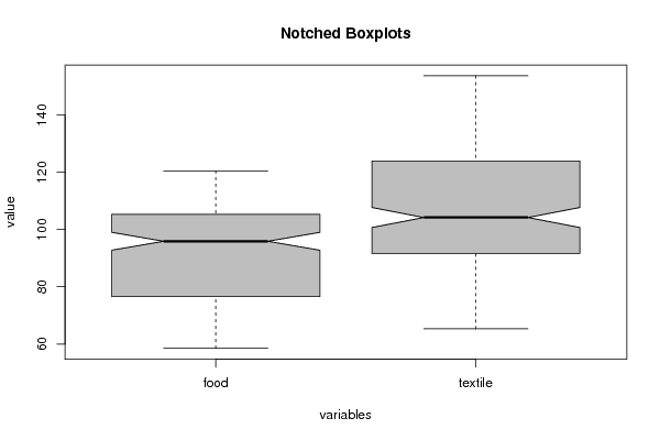
Title produced by software

Notched Boxplots

Date of computation

Wed, 13 Dec 2017 14:27:09 +0100

Cite this page as follows

Statistical Computations at FreeStatistics.org, Office for Research Development and Education, URL https://freestatistics.org/blog/index.php?v=date/2017/Dec/13/t1513171641vh8nw54b8rp7edf.htm/, Retrieved Wed, 15 May 2024 03:38:37 +0000

Statistical Computations at FreeStatistics.org, Office for Research Development and Education, URL https://freestatistics.org/blog/index.php?pk=309295, Retrieved Wed, 15 May 2024 03:38:37 +0000

QR Codes:

Paste this QR Code to cite your computation.

Original text written by user:

IsPrivate?

No (this computation is public)

User-defined keywords

Estimated Impact

Family? (F = Feedback message, R = changed R code, M = changed R Module, P = changed Parameters, D = changed Data)

-       [Notched Boxplots] [] [2017-12-13 13:27:09] [c34712453b62a314277c4dd71143a000] [Current]

Feedback Forum

Post a new message

Dataseries X:

Download CSV

Histogram

Boxplots

58.5	120.7
59.8	134.1
64.6	143.6
62.2	115.1
68	135.1
64.3	123.6
58.9	110.7
64.8	104.3
67.5	143.7
76.2	149.7
73.7	143.3
70.4	115.3
67.7	136.2
63.7	137.4
72.4	147.6
66	123.7
70.1	131.6
70.4	132.7
66.6	123
72.6	108.2
74	140.9
79	149.2
76.1	134.5
72.3	103.2
71.6	136.2
67.2	135.6
73.8	139.7
70.8	131
71.4	124.4
70.4	123.6
70.7	125.1
70.6	106.2
75.5	144.4
82.1	153.7
74.3	131.5
76.3	105.5
74.5	136.3
71.1	133.4
73.3	129.8
73.8	129.1
69	113
71.1	117.1
71.9	115.4
69	96.5
77.3	141
82.8	141.3
74	121
77.6	106
72.3	121.9
70.7	122.4
81	137.4
76.4	118.9
72.3	106.7
79.5	126.5
73.3	110.8
74.5	99.3
82.7	138.7
83.8	128.9
81.6	121.9
85.5	106
76.7	113.1
71.8	124.2
80.2	129.2
76.8	116.5
76.1	105.7
80.7	122
71.3	105.1
80.9	100.8
85	131.8
84.5	119.9
87.7	127.1
87.7	107.1
80.2	115.8
74.4	122.9
85.8	137.5
77	108.9
84.5	114.9
83.6	129.7
77.7	111.8
85.7	103.4
87.9	140.3
93.7	140.7
92.3	136.1
87	106.3
89.1	127.7
81.3	136.4
92.7	145.1
83.9	116.5
87.3	117.6
89.1	129
86.9	117.4
91.7	107.2
93	130.9
105.3	145.1
101.6	127.8
94.2	96.6
100.5	126
95.8	130.1
95.8	124.5
102.1	137.4
96	105.6
96.8	113.3
98.9	108.4
93.4	83.5
105.5	116.2
110.9	115.6
98.6	95.6
102.6	83.5
93.5	95.3
90.8	95.8
99.7	100.4
97.8	90.9
91.1	80
98.1	93.8
96	92.3
93.5	74.3
101.2	101.4
105.2	103.7
98.9	92.4
101.3	83.4
92.1	91.6
90.6	101.2
105.4	109.2
98.4	100.3
92.7	91
101.2	110.9
93.4	96.3
98.3	80.4
104.3	114.5
107	109.9
107.7	104.1
108.9	90.7
99.6	94.6
96.1	100.4
109	115.9
99.5	94.4
104.6	102.5
99.9	97.3
94.1	90
105.3	81.1
110.4	107.3
110.5	100.5
110	95.4
108.5	81.1
104.3	92.2
101.2	98.4
109.2	98.6
99.6	81.4
105.6	85.5
106.2	90.4
102.2	83.7
107.5	73.3
105.8	89.8
120.5	101.6
113.2	87.5
104.3	65.3
107.7	87.1
99.2	89.9
105.1	91.5
104.3	84.7
106.1	84.1
100.8	86.7
106.7	89.6
101.6	65.7
104.4	92.9
114.8	97.7
105.4	84.4
104	68.1
102	95
96.5	96.3
102.3	94.7
105.3	89.7
101.9	81.3
102.2	89.3
102.8	94.2
100.4	68.7
110.7	105.7
116.4	102
106	84.3
109.2	74.9
103	92.9
99.8	100.4
109.8	99.4
107.3	94.6
101.2	84
111.8	102.2
106.9	91.4
103.5	79.8
113.1	101
119.4	97.5
113.3	87.8
115	77.1
104.7	89.6
107.2	100.9
116.6	97.8
111.3	90.5
111.4	84.2
115	96.8
102.4	82.9
111.4	75.6
113.2	91.9
112.9	85.4
114.2	90.4
115.6	74
107.1	93.1
102.3	94.9
117.9	102.9
105.8	80.7
114.3	91.7
113.1	95.5
102.9	84.8
112.2	74.4

Summary of computational transaction
Raw Input	view raw input (R code)
Raw Output	view raw output of R engine
Computing time	2 seconds
R Server	Big Analytics Cloud Computing Center

\begin{tabular}{lllllllll}
\hline
Summary of computational transaction \tabularnewline
Raw Input view raw input (R code)  \tabularnewline
Raw Outputview raw output of R engine  \tabularnewline
Computing time2 seconds \tabularnewline
R ServerBig Analytics Cloud Computing Center \tabularnewline
\hline
\end{tabular}
%Source: https://freestatistics.org/blog/index.php?pk=309295&T=0

[TABLE]
[ROW]

Summary of computational transaction[/C][/ROW] [ROW]

Raw Input[/C]

view raw input (R code) [/C][/ROW] [ROW]

Raw Output[/C]

view raw output of R engine [/C][/ROW] [ROW]

Computing time[/C]

2 seconds[/C][/ROW] [ROW]

R Server[/C]

Big Analytics Cloud Computing Center[/C][/ROW] [/TABLE] Source: https://freestatistics.org/blog/index.php?pk=309295&T=0

Globally Unique Identifier (entire table): ba.freestatistics.org/blog/index.php?pk=309295&T=0

As an alternative you can also use a QR Code:

The GUIDs for individual cells are displayed in the table below:

Summary of computational transaction
Raw Input	view raw input (R code)
Raw Output	view raw output of R engine
Computing time	2 seconds
R Server	Big Analytics Cloud Computing Center

Boxplot statistics
Variable	lower whisker	lower hinge	median	upper hinge	upper whisker
food	58.5	76.55	95.9	105.3	120.5
textile	65.3	91.65	104.2	123.95	153.7

\begin{tabular}{lllllllll}
\hline
Boxplot statistics \tabularnewline
Variable & lower whisker & lower hinge & median & upper hinge & upper whisker \tabularnewline
food & 58.5 & 76.55 & 95.9 & 105.3 & 120.5 \tabularnewline
textile & 65.3 & 91.65 & 104.2 & 123.95 & 153.7 \tabularnewline
\hline
\end{tabular}
%Source: https://freestatistics.org/blog/index.php?pk=309295&T=1

[TABLE]
[ROW][C]Boxplot statistics[/C][/ROW]
[ROW][C]Variable[/C][C]lower whisker[/C][C]lower hinge[/C][C]median[/C][C]upper hinge[/C][C]upper whisker[/C][/ROW]
[ROW][C]food[/C][C]58.5[/C][C]76.55[/C][C]95.9[/C][C]105.3[/C][C]120.5[/C][/ROW]
[ROW][C]textile[/C][C]65.3[/C][C]91.65[/C][C]104.2[/C][C]123.95[/C][C]153.7[/C][/ROW]
[/TABLE]
Source: https://freestatistics.org/blog/index.php?pk=309295&T=1

Globally Unique Identifier (entire table): ba.freestatistics.org/blog/index.php?pk=309295&T=1

As an alternative you can also use a QR Code:

The GUIDs for individual cells are displayed in the table below:

Boxplot statistics
Variable	lower whisker	lower hinge	median	upper hinge	upper whisker
food	58.5	76.55	95.9	105.3	120.5
textile	65.3	91.65	104.2	123.95	153.7

Boxplot Notches
Variable	lower bound	median	upper bound
food	92.7801981913154	95.9	99.0198018086846
textile	100.694970489721	104.2	107.705029510279

\begin{tabular}{lllllllll}
\hline
Boxplot Notches \tabularnewline
Variable & lower bound & median & upper bound \tabularnewline
food & 92.7801981913154 & 95.9 & 99.0198018086846 \tabularnewline
textile & 100.694970489721 & 104.2 & 107.705029510279 \tabularnewline
\hline
\end{tabular}
%Source: https://freestatistics.org/blog/index.php?pk=309295&T=2

[TABLE]
[ROW][C]Boxplot Notches[/C][/ROW]
[ROW][C]Variable[/C][C]lower bound[/C][C]median[/C][C]upper bound[/C][/ROW]
[ROW][C]food[/C][C]92.7801981913154[/C][C]95.9[/C][C]99.0198018086846[/C][/ROW]
[ROW][C]textile[/C][C]100.694970489721[/C][C]104.2[/C][C]107.705029510279[/C][/ROW]
[/TABLE]
Source: https://freestatistics.org/blog/index.php?pk=309295&T=2

Globally Unique Identifier (entire table): ba.freestatistics.org/blog/index.php?pk=309295&T=2

As an alternative you can also use a QR Code:

The GUIDs for individual cells are displayed in the table below:

Boxplot Notches
Variable	lower bound	median	upper bound
food	92.7801981913154	95.9	99.0198018086846
textile	100.694970489721	104.2	107.705029510279

Figure 1

PNG link

Postscript link

PDF link

Parameters (Session):

par1 = 1 ; par2 = 2 ; par3 = 0.95 ; par4 = two.sided ; par5 = unpaired ; par6 = 0.0 ;

Parameters (R input):

par1 = grey ; par2 = no ;

R code (references can be found in the software module):

if(par2=='yes') {
z <- na.omit(as.data.frame(t(y)))
} else {
z <- as.data.frame(t(y))
}
bitmap(file='test1.png')
(r<-boxplot(z ,xlab=xlab,ylab=ylab,main=main,notch=TRUE,col=par1))
dev.off()
load(file='createtable')
a<-table.start()
a<-table.row.start(a)
a<-table.element(a,'Boxplot statistics',6,TRUE)
a<-table.row.end(a)
a<-table.row.start(a)
a<-table.element(a,'Variable',1,TRUE)
a<-table.element(a,'lower whisker',1,TRUE)
a<-table.element(a,'lower hinge',1,TRUE)
a<-table.element(a,'median',1,TRUE)
a<-table.element(a,'upper hinge',1,TRUE)
a<-table.element(a,'upper whisker',1,TRUE)
a<-table.row.end(a)
for (i in 1:length(y[,1]))
{
a<-table.row.start(a)
a<-table.element(a,dimnames(t(x))[[2]][i],1,TRUE)
for (j in 1:5)
{
a<-table.element(a,r$stats[j,i])
}
a<-table.row.end(a)
}
a<-table.end(a)
table.save(a,file='mytable.tab')
a<-table.start()
a<-table.row.start(a)
a<-table.element(a,'Boxplot Notches',4,TRUE)
a<-table.row.end(a)
a<-table.row.start(a)
a<-table.element(a,'Variable',1,TRUE)
a<-table.element(a,'lower bound',1,TRUE)
a<-table.element(a,'median',1,TRUE)
a<-table.element(a,'upper bound',1,TRUE)
a<-table.row.end(a)
for (i in 1:length(y[,1]))
{
a<-table.row.start(a)
a<-table.element(a,dimnames(t(x))[[2]][i],1,TRUE)
a<-table.element(a,r$conf[1,i])
a<-table.element(a,r$stats[3,i])
a<-table.element(a,r$conf[2,i])
a<-table.row.end(a)
}
a<-table.end(a)
table.save(a,file='mytable1.tab')

Free Statistics

Description of Statistical Computation

Tree of Dependent Computations

Dataset

Tables (Output of Computation)

Figures (Output of Computation)

Input Parameters & R Code