Free Statistics

of Irreproducible Research!

Author's title

Author*The author of this computation has been verified*
R Software Modulerwasp_correlation.wasp
Title produced by softwarePearson Correlation
Date of computationWed, 06 Dec 2017 14:12:13 +0100
Cite this page as followsStatistical Computations at FreeStatistics.org, Office for Research Development and Education, URL https://freestatistics.org/blog/index.php?v=date/2017/Dec/06/t1512568037ftu4hyngmzmb1xt.htm/, Retrieved Tue, 14 May 2024 13:34:03 +0000
Statistical Computations at FreeStatistics.org, Office for Research Development and Education, URL https://freestatistics.org/blog/index.php?pk=308614, Retrieved Tue, 14 May 2024 13:34:03 +0000
QR Codes:

Original text written by user:
IsPrivate?No (this computation is public)
User-defined keywords
Estimated Impact101
Family? (F = Feedback message, R = changed R code, M = changed R Module, P = changed Parameters, D = changed Data)
-       [Pearson Correlation] [Pearson correlati...] [2017-12-06 13:12:13] [09ca0998dffcdc3bb8b8a63ab2cdd9f2] [Current]
Feedback Forum

Post a new message
Dataseries X:
68
39
32
62
33
52
62
77
76
41
48
63
30
78
19
31
66
35
42
45
21
25
44
69
54
74
80
42
61
41
46
39
34
51
42
31
39
20
49
53
31
39
54
49
34
46
55
42
50
13
37
25
30
28
45
35
28
41
6
45
73
17
40
64
37
25
65
100
28
35
56
29
43
59
50
59
27
61
28
51
35
29
48
25
44
64
32
20
28
34
31
26
58
23
21
21
33
16
20
37
35
33
27
41
40
35
28
32
22
44
27
17
12
45
37
37
108
10
68
72
143
9
55
17
37
27
37
58
66
21
19
78
35
48
27
43
30
25
69
72
23
13
61
43
51
67
36
44
45
34
36
72
39
43
25
56
80
40
73
34
72
42
61
23
74
16
66
9
41
57
48
51
53
29
29
55
54
43
51
20
79
39
61
55
30
55
22
37
2
38
27
56
25
39
33
43
57
43
23
44
54
28
36
39
16
23
40
24
78
57
37
27
61
27
69
34
44
34
39
51
34
31
13
12
51
24
19
30
81
42
22
85
27
25
22
19
14
45
45
28
51
41
31
74
19
51
73
24
61
23
14
54
51
62
36
59
24
26
54
39
16
36
31
31
42
39
25
31
38
31
17
22
55
62
51
30
49
16
Dataseries Y:
12.9
12.2
12.8
7.4
6.7
12.6
14.8
13.3
11.1
8.2
11.4
6.4
10.6
12
6.3
11.3
11.9
9.3
9.6
10
6.4
13.8
10.8
13.8
11.7
10.9
16.1
13.4
9.9
11.5
8.3
11.7
9
9.7
10.8
10.3
10.4
12.7
9.3
11.8
5.9
11.4
13
10.8
12.3
11.3
11.8
7.9
12.7
12.3
11.6
6.7
10.9
12.1
13.3
10.1
5.7
14.3
8
13.3
9.3
12.5
7.6
15.9
9.2
9.1
11.1
13
14.5
12.2
12.3
11.4
8.8
14.6
12.6
13
12.6
13.2
9.9
7.7
10.5
13.4
10.9
4.3
10.3
11.8
11.2
11.4
8.6
13.2
12.6
5.6
9.9
8.8
7.7
9
7.3
11.4
13.6
7.9
10.7
10.3
8.3
9.6
14.2
8.5
13.5
4.9
6.4
9.6
11.6
11.1
4.35
12.7
18.1
17.85
16.6
12.6
17.1
19.1
16.1
13.35
18.4
14.7
10.6
12.6
16.2
13.6
18.9
14.1
14.5
16.15
14.75
14.8
12.45
12.65
17.35
8.6
18.4
16.1
11.6
17.75
15.25
17.65
16.35
17.65
13.6
14.35
14.75
18.25
9.9
16
18.25
16.85
14.6
13.85
18.95
15.6
14.85
11.75
18.45
15.9
17.1
16.1
19.9
10.95
18.45
15.1
15
11.35
15.95
18.1
14.6
15.4
15.4
17.6
13.35
19.1
15.35
7.6
13.4
13.9
19.1
15.25
12.9
16.1
17.35
13.15
12.15
12.6
10.35
15.4
9.6
18.2
13.6
14.85
14.75
14.1
14.9
16.25
19.25
13.6
13.6
15.65
12.75
14.6
9.85
12.65
19.2
16.6
11.2
15.25
11.9
13.2
16.35
12.4
15.85
18.15
11.15
15.65
17.75
7.65
12.35
15.6
19.3
15.2
17.1
15.6
18.4
19.05
18.55
19.1
13.1
12.85
9.5
4.5
11.85
13.6
11.7
12.4
13.35
11.4
14.9
19.9
11.2
14.6
17.6
14.05
16.1
13.35
11.85
11.95
14.75
15.15
13.2
16.85
7.85
7.7
12.6
7.85
10.95
12.35
9.95
14.9
16.65
13.4
13.95
15.7
16.85
10.95
15.35
12.2
15.1
17.75
15.2
14.6
16.65
8.1


Summary of computational transaction
Raw Input view raw input (R code)
Raw Outputview raw output of R engine
Computing time6 seconds
R ServerBig Analytics Cloud Computing Center

\begin{tabular}{lllllllll}
\hline
Summary of computational transaction \tabularnewline
Raw Input view raw input (R code)  \tabularnewline
Raw Outputview raw output of R engine  \tabularnewline
Computing time6 seconds \tabularnewline
R ServerBig Analytics Cloud Computing Center \tabularnewline
\hline
\end{tabular}
%Source: https://freestatistics.org/blog/index.php?pk=308614&T=0

[TABLE]
[ROW]
Summary of computational transaction[/C][/ROW] [ROW]Raw Input[/C] view raw input (R code) [/C][/ROW] [ROW]Raw Output[/C]view raw output of R engine [/C][/ROW] [ROW]Computing time[/C]6 seconds[/C][/ROW] [ROW]R Server[/C]Big Analytics Cloud Computing Center[/C][/ROW] [/TABLE] Source: https://freestatistics.org/blog/index.php?pk=308614&T=0

Globally Unique Identifier (entire table): ba.freestatistics.org/blog/index.php?pk=308614&T=0

As an alternative you can also use a QR Code:  

The GUIDs for individual cells are displayed in the table below:

Summary of computational transaction
Raw Input view raw input (R code)
Raw Outputview raw output of R engine
Computing time6 seconds
R ServerBig Analytics Cloud Computing Center


Pearson Product Moment Correlation - Ungrouped Data
StatisticVariable XVariable Y
Mean41.43165467625912.975
Biased Variance362.25252316132711.4802293165468
Biased Standard Deviation19.03293259488213.3882487093699
Covariance23.6657039711191
Correlation0.36565659412503
Determination0.133704744827117
T-Test6.52672001968661
p-value (2 sided)3.20865880255605e-10
p-value (1 sided)1.60432940127803e-10
95% CI of Correlation[0.259161945864746, 0.463366967345079]
Degrees of Freedom276
Number of Observations278

\begin{tabular}{lllllllll}
\hline
Pearson Product Moment Correlation - Ungrouped Data \tabularnewline
Statistic & Variable X & Variable Y \tabularnewline
Mean & 41.431654676259 & 12.975 \tabularnewline
Biased Variance & 362.252523161327 & 11.4802293165468 \tabularnewline
Biased Standard Deviation & 19.0329325948821 & 3.3882487093699 \tabularnewline
Covariance & 23.6657039711191 \tabularnewline
Correlation & 0.36565659412503 \tabularnewline
Determination & 0.133704744827117 \tabularnewline
T-Test & 6.52672001968661 \tabularnewline
p-value (2 sided) & 3.20865880255605e-10 \tabularnewline
p-value (1 sided) & 1.60432940127803e-10 \tabularnewline
95% CI of Correlation & [0.259161945864746, 0.463366967345079] \tabularnewline
Degrees of Freedom & 276 \tabularnewline
Number of Observations & 278 \tabularnewline
\hline
\end{tabular}
%Source: https://freestatistics.org/blog/index.php?pk=308614&T=1

[TABLE]
[ROW][C]Pearson Product Moment Correlation - Ungrouped Data[/C][/ROW]
[ROW][C]Statistic[/C][C]Variable X[/C][C]Variable Y[/C][/ROW]
[ROW][C]Mean[/C][C]41.431654676259[/C][C]12.975[/C][/ROW]
[ROW][C]Biased Variance[/C][C]362.252523161327[/C][C]11.4802293165468[/C][/ROW]
[ROW][C]Biased Standard Deviation[/C][C]19.0329325948821[/C][C]3.3882487093699[/C][/ROW]
[ROW][C]Covariance[/C][C]23.6657039711191[/C][/ROW]
[ROW][C]Correlation[/C][C]0.36565659412503[/C][/ROW]
[ROW][C]Determination[/C][C]0.133704744827117[/C][/ROW]
[ROW][C]T-Test[/C][C]6.52672001968661[/C][/ROW]
[ROW][C]p-value (2 sided)[/C][C]3.20865880255605e-10[/C][/ROW]
[ROW][C]p-value (1 sided)[/C][C]1.60432940127803e-10[/C][/ROW]
[ROW][C]95% CI of Correlation[/C][C][0.259161945864746, 0.463366967345079][/C][/ROW]
[ROW][C]Degrees of Freedom[/C][C]276[/C][/ROW]
[ROW][C]Number of Observations[/C][C]278[/C][/ROW]
[/TABLE]
Source: https://freestatistics.org/blog/index.php?pk=308614&T=1

Globally Unique Identifier (entire table): ba.freestatistics.org/blog/index.php?pk=308614&T=1

As an alternative you can also use a QR Code:  

The GUIDs for individual cells are displayed in the table below:

Pearson Product Moment Correlation - Ungrouped Data
StatisticVariable XVariable Y
Mean41.43165467625912.975
Biased Variance362.25252316132711.4802293165468
Biased Standard Deviation19.03293259488213.3882487093699
Covariance23.6657039711191
Correlation0.36565659412503
Determination0.133704744827117
T-Test6.52672001968661
p-value (2 sided)3.20865880255605e-10
p-value (1 sided)1.60432940127803e-10
95% CI of Correlation[0.259161945864746, 0.463366967345079]
Degrees of Freedom276
Number of Observations278


Normality Tests
> jarque.x
	Jarque-Bera Normality Test
data:  x
JB = 115.67, p-value < 2.2e-16
alternative hypothesis: greater
> jarque.y
	Jarque-Bera Normality Test
data:  y
JB = 3.2947, p-value = 0.1926
alternative hypothesis: greater
> ad.x
	Anderson-Darling normality test
data:  x
A = 2.3388, p-value = 6.19e-06
> ad.y
	Anderson-Darling normality test
data:  y
A = 0.42625, p-value = 0.3124

\begin{tabular}{lllllllll}
\hline
Normality Tests \tabularnewline
> jarque.x
	Jarque-Bera Normality Test
data:  x
JB = 115.67, p-value < 2.2e-16
alternative hypothesis: greater
\tabularnewline
> jarque.y
	Jarque-Bera Normality Test
data:  y
JB = 3.2947, p-value = 0.1926
alternative hypothesis: greater
\tabularnewline
> ad.x
	Anderson-Darling normality test
data:  x
A = 2.3388, p-value = 6.19e-06
\tabularnewline
> ad.y
	Anderson-Darling normality test
data:  y
A = 0.42625, p-value = 0.3124
\tabularnewline \hline \end{tabular} %Source: https://freestatistics.org/blog/index.php?pk=308614&T=2

[TABLE]
[ROW][C]Normality Tests[/C][/ROW]
[ROW][C]
> jarque.x
	Jarque-Bera Normality Test
data:  x
JB = 115.67, p-value < 2.2e-16
alternative hypothesis: greater
[/C][/ROW] [ROW][C]
> jarque.y
	Jarque-Bera Normality Test
data:  y
JB = 3.2947, p-value = 0.1926
alternative hypothesis: greater
[/C][/ROW] [ROW][C]
> ad.x
	Anderson-Darling normality test
data:  x
A = 2.3388, p-value = 6.19e-06
[/C][/ROW] [ROW][C]
> ad.y
	Anderson-Darling normality test
data:  y
A = 0.42625, p-value = 0.3124
[/C][/ROW] [/TABLE] Source: https://freestatistics.org/blog/index.php?pk=308614&T=2

Globally Unique Identifier (entire table): ba.freestatistics.org/blog/index.php?pk=308614&T=2

As an alternative you can also use a QR Code:  

The GUIDs for individual cells are displayed in the table below:

Normality Tests
> jarque.x
	Jarque-Bera Normality Test
data:  x
JB = 115.67, p-value < 2.2e-16
alternative hypothesis: greater
> jarque.y
	Jarque-Bera Normality Test
data:  y
JB = 3.2947, p-value = 0.1926
alternative hypothesis: greater
> ad.x
	Anderson-Darling normality test
data:  x
A = 2.3388, p-value = 6.19e-06
> ad.y
	Anderson-Darling normality test
data:  y
A = 0.42625, p-value = 0.3124


Parameters (Session):
Parameters (R input):
R code (references can be found in the software module):
library(psychometric)
x <- x[!is.na(y)]
y <- y[!is.na(y)]
y <- y[!is.na(x)]
x <- x[!is.na(x)]
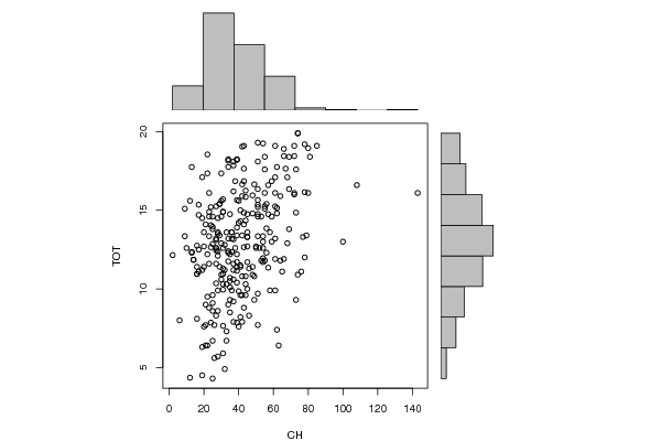
bitmap(file='test1.png')
histx <- hist(x, plot=FALSE)
histy <- hist(y, plot=FALSE)
maxcounts <- max(c(histx$counts, histx$counts))
xrange <- c(min(x),max(x))
yrange <- c(min(y),max(y))
nf <- layout(matrix(c(2,0,1,3),2,2,byrow=TRUE), c(3,1), c(1,3), TRUE)
par(mar=c(4,4,1,1))
plot(x, y, xlim=xrange, ylim=yrange, xlab=xlab, ylab=ylab, sub=main)
par(mar=c(0,4,1,1))
barplot(histx$counts, axes=FALSE, ylim=c(0, maxcounts), space=0)
par(mar=c(4,0,1,1))
barplot(histy$counts, axes=FALSE, xlim=c(0, maxcounts), space=0, horiz=TRUE)
dev.off()
lx = length(x)
makebiased = (lx-1)/lx
varx = var(x)*makebiased
vary = var(y)*makebiased
corxy <- cor.test(x,y,method='pearson', na.rm = T)
cxy <- as.matrix(corxy$estimate)[1,1]
load(file='createtable')
a<-table.start()
a<-table.row.start(a)
a<-table.element(a,'Pearson Product Moment Correlation - Ungrouped Data',3,TRUE)
a<-table.row.end(a)
a<-table.row.start(a)
a<-table.element(a,'Statistic',1,TRUE)
a<-table.element(a,'Variable X',1,TRUE)
a<-table.element(a,'Variable Y',1,TRUE)
a<-table.row.end(a)
a<-table.row.start(a)
a<-table.element(a,'Mean',header=TRUE)
a<-table.element(a,mean(x))
a<-table.element(a,mean(y))
a<-table.row.end(a)
a<-table.row.start(a)
a<-table.element(a,'Biased Variance',header=TRUE)
a<-table.element(a,varx)
a<-table.element(a,vary)
a<-table.row.end(a)
a<-table.row.start(a)
a<-table.element(a,'Biased Standard Deviation',header=TRUE)
a<-table.element(a,sqrt(varx))
a<-table.element(a,sqrt(vary))
a<-table.row.end(a)
a<-table.row.start(a)
a<-table.element(a,'Covariance',header=TRUE)
a<-table.element(a,cov(x,y),2)
a<-table.row.end(a)
a<-table.row.start(a)
a<-table.element(a,'Correlation',header=TRUE)
a<-table.element(a,cxy,2)
a<-table.row.end(a)
a<-table.row.start(a)
a<-table.element(a,'Determination',header=TRUE)
a<-table.element(a,cxy*cxy,2)
a<-table.row.end(a)
a<-table.row.start(a)
a<-table.element(a,'T-Test',header=TRUE)
a<-table.element(a,as.matrix(corxy$statistic)[1,1],2)
a<-table.row.end(a)
a<-table.row.start(a)
a<-table.element(a,'p-value (2 sided)',header=TRUE)
a<-table.element(a,(p2 <- as.matrix(corxy$p.value)[1,1]),2)
a<-table.row.end(a)
a<-table.row.start(a)
a<-table.element(a,'p-value (1 sided)',header=TRUE)
a<-table.element(a,p2/2,2)
a<-table.row.end(a)
a<-table.row.start(a)
a<-table.element(a,'95% CI of Correlation',header=TRUE)
a<-table.element(a,paste('[',CIr(r=cxy, n = lx, level = .95)[1],', ', CIr(r=cxy, n = lx, level = .95)[2],']',sep=''),2)
a<-table.row.end(a)
a<-table.row.start(a)
a<-table.element(a,'Degrees of Freedom',header=TRUE)
a<-table.element(a,lx-2,2)
a<-table.row.end(a)
a<-table.row.start(a)
a<-table.element(a,'Number of Observations',header=TRUE)
a<-table.element(a,lx,2)
a<-table.row.end(a)
a<-table.end(a)
table.save(a,file='mytable.tab')
library(moments)
library(nortest)
jarque.x <- jarque.test(x)
jarque.y <- jarque.test(y)
if(lx>7) {
ad.x <- ad.test(x)
ad.y <- ad.test(y)
}
a<-table.start()
a<-table.row.start(a)
a<-table.element(a,'Normality Tests',1,TRUE)
a<-table.row.end(a)
a<-table.row.start(a)
a<-table.element(a,paste('
',RC.texteval('jarque.x'),'
',sep=''))
a<-table.row.end(a)
a<-table.row.start(a)
a<-table.element(a,paste('
',RC.texteval('jarque.y'),'
',sep=''))
a<-table.row.end(a)
if(lx>7) {
a<-table.row.start(a)
a<-table.element(a,paste('
',RC.texteval('ad.x'),'
',sep=''))
a<-table.row.end(a)
a<-table.row.start(a)
a<-table.element(a,paste('
',RC.texteval('ad.y'),'
',sep=''))
a<-table.row.end(a)
}
a<-table.end(a)
table.save(a,file='mytable1.tab')
library(car)
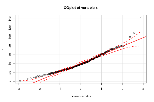
bitmap(file='test2.png')
qqPlot(x,main='QQplot of variable x')
dev.off()
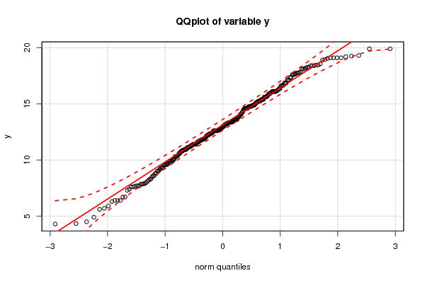
bitmap(file='test3.png')
qqPlot(y,main='QQplot of variable y')
dev.off()