Repository of Reproducible Computations

Free Statistics

of Irreproducible Research!

Author's title

Author

*Unverified author*

R Software Module

rwasp_decompose.wasp

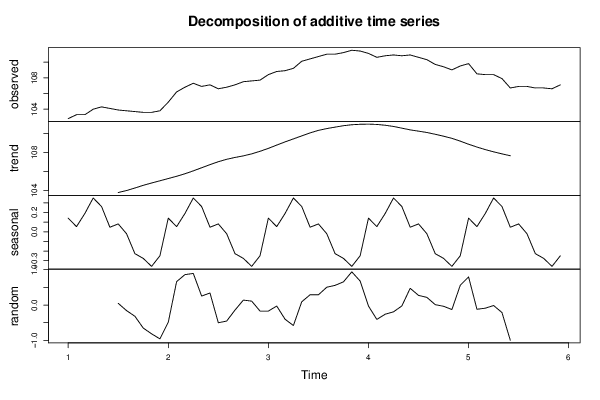
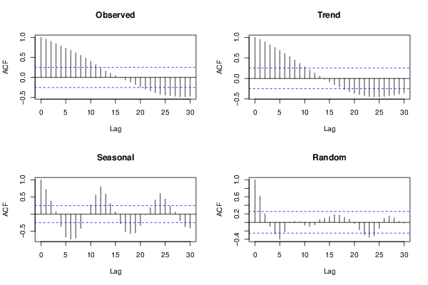
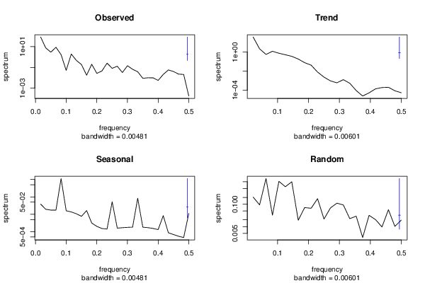
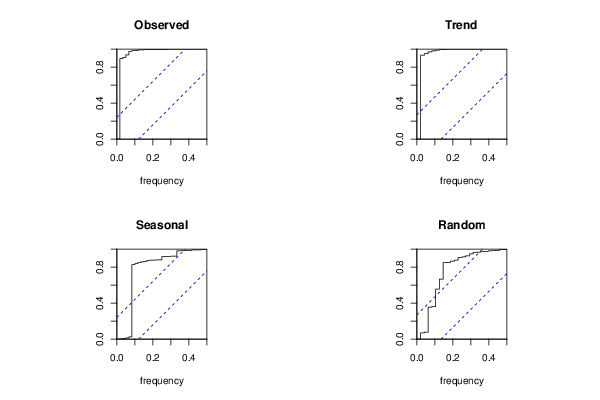
Title produced by software

Classical Decomposition

Date of computation

Sat, 29 Apr 2017 10:28:00 +0100

Cite this page as follows

Statistical Computations at FreeStatistics.org, Office for Research Development and Education, URL https://freestatistics.org/blog/index.php?v=date/2017/Apr/29/t1493458148sk5jvrli306spyf.htm/, Retrieved Mon, 13 May 2024 06:51:02 +0200

Statistical Computations at FreeStatistics.org, Office for Research Development and Education, URL https://freestatistics.org/blog/index.php?pk=, Retrieved Mon, 13 May 2024 06:51:02 +0200

QR Codes:

Paste this QR Code to cite your computation.

Original text written by user:

IsPrivate?

No (this computation is public)

User-defined keywords

Estimated Impact

Dataseries X:

Download CSV

Histogram

Boxplots

Summary of computational transaction
Raw Input	view raw input (R code)
Raw Output	view raw output of R engine
Computing time	2 seconds
R Server	'Herman Ole Andreas Wold' @ wold.wessa.net

\begin{tabular}{lllllllll}
\hline
Summary of computational transaction \tabularnewline
Raw Input & view raw input (R code)  \tabularnewline
Raw Output & view raw output of R engine  \tabularnewline
Computing time & 2 seconds \tabularnewline
R Server & 'Herman Ole Andreas Wold' @ wold.wessa.net \tabularnewline
\hline
\end{tabular}
%Source: https://freestatistics.org/blog/index.php?pk=&T=0

[TABLE]
[ROW][C]Summary of computational transaction[/C][/ROW]
[ROW][C]Raw Input[/C][C]view raw input (R code) [/C][/ROW]
[ROW][C]Raw Output[/C][C]view raw output of R engine [/C][/ROW]
[ROW][C]Computing time[/C][C]2 seconds[/C][/ROW]
[ROW][C]R Server[/C][C]'Herman Ole Andreas Wold' @ wold.wessa.net[/C][/ROW]
[/TABLE]
Source: https://freestatistics.org/blog/index.php?pk=&T=0

Globally Unique Identifier (entire table): ba.freestatistics.org/blog/index.php?pk=&T=0

As an alternative you can also use a QR Code:

The GUIDs for individual cells are displayed in the table below:

Summary of computational transaction
Raw Input	view raw input (R code)
Raw Output	view raw output of R engine
Computing time	2 seconds
R Server	'Herman Ole Andreas Wold' @ wold.wessa.net

Classical Decomposition by Moving Averages
t	Observations	Fit	Trend	Seasonal	Random
1	102.8	NA	NA	0.142535	NA
2	103.3	NA	NA	0.0539931	NA
3	103.3	NA	NA	0.190451	NA
4	104	NA	NA	0.35191	NA
5	104.3	NA	NA	0.263368	NA
6	104.1	NA	NA	0.0477431	NA
7	103.9	103.853	103.771	0.0821181	0.0470486
8	103.8	103.959	103.979	-0.0199653	-0.159201
9	103.7	104.019	104.246	-0.227257	-0.318576
10	103.6	104.253	104.529	-0.276215	-0.652951
11	103.6	104.415	104.775	-0.359549	-0.815451
12	103.8	104.759	105.008	-0.249132	-0.959201
13	104.9	105.388	105.246	0.142535	-0.488368
14	106.2	105.537	105.483	0.0539931	0.662674
15	106.8	105.94	105.75	0.190451	0.859549
16	107.3	106.406	106.054	0.35191	0.893924
17	106.9	106.647	106.383	0.263368	0.253299
18	107.1	106.76	106.712	0.0477431	0.339757
19	106.6	107.103	107.021	0.0821181	-0.502951
20	106.8	107.255	107.275	-0.0199653	-0.455035
21	107.1	107.244	107.471	-0.227257	-0.143576
22	107.5	107.361	107.637	-0.276215	0.138715
23	107.6	107.49	107.85	-0.359549	0.109549
24	107.7	107.872	108.121	-0.249132	-0.171701
25	108.4	108.572	108.429	0.142535	-0.171701
26	108.8	108.829	108.775	0.0539931	-0.0289931
27	108.9	109.303	109.112	0.190451	-0.402951
28	109.2	109.781	109.429	0.35191	-0.581076
29	110.1	110.009	109.746	0.263368	0.0907986
30	110.4	110.11	110.062	0.0477431	0.289757
31	110.7	110.411	110.329	0.0821181	0.288715
32	111	110.497	110.517	-0.0199653	0.503299
33	111	110.444	110.671	-0.227257	0.556424
34	111.2	110.545	110.821	-0.276215	0.655382
35	111.5	110.561	110.921	-0.359549	0.938715
36	111.4	110.722	110.971	-0.249132	0.678299
37	111.1	111.13	110.988	0.142535	-0.0300347
38	110.6	111.008	110.954	0.0539931	-0.40816
39	110.8	111.061	110.871	0.190451	-0.261285
40	110.9	111.094	110.742	0.35191	-0.193576
41	110.8	110.826	110.562	0.263368	-0.0258681
42	110.9	110.427	110.379	0.0477431	0.47309
43	110.6	110.328	110.246	0.0821181	0.272049
44	110.3	110.084	110.104	-0.0199653	0.215799
45	109.7	109.689	109.917	-0.227257	0.0105903
46	109.4	109.436	109.713	-0.276215	-0.0362847
47	109	109.128	109.487	-0.359549	-0.127951
48	109.5	108.943	109.192	-0.249132	0.557465
49	109.8	109.005	108.862	0.142535	0.794965
50	108.5	108.621	108.567	0.0539931	-0.12066
51	108.4	108.49	108.3	0.190451	-0.0904514
52	108.4	108.414	108.062	0.35191	-0.0144097
53	107.9	108.113	107.85	0.263368	-0.213368
54	106.7	107.698	107.65	0.0477431	-0.997743
55	106.9	NA	NA	0.0821181	NA
56	106.9	NA	NA	-0.0199653	NA
57	106.7	NA	NA	-0.227257	NA
58	106.7	NA	NA	-0.276215	NA
59	106.6	NA	NA	-0.359549	NA
60	107.1	NA	NA	-0.249132	NA

\begin{tabular}{lllllllll}
\hline
Classical Decomposition by Moving Averages \tabularnewline
t & Observations & Fit & Trend & Seasonal & Random \tabularnewline
1 & 102.8 & NA & NA & 0.142535 & NA \tabularnewline
2 & 103.3 & NA & NA & 0.0539931 & NA \tabularnewline
3 & 103.3 & NA & NA & 0.190451 & NA \tabularnewline
4 & 104 & NA & NA & 0.35191 & NA \tabularnewline
5 & 104.3 & NA & NA & 0.263368 & NA \tabularnewline
6 & 104.1 & NA & NA & 0.0477431 & NA \tabularnewline
7 & 103.9 & 103.853 & 103.771 & 0.0821181 & 0.0470486 \tabularnewline
8 & 103.8 & 103.959 & 103.979 & -0.0199653 & -0.159201 \tabularnewline
9 & 103.7 & 104.019 & 104.246 & -0.227257 & -0.318576 \tabularnewline
10 & 103.6 & 104.253 & 104.529 & -0.276215 & -0.652951 \tabularnewline
11 & 103.6 & 104.415 & 104.775 & -0.359549 & -0.815451 \tabularnewline
12 & 103.8 & 104.759 & 105.008 & -0.249132 & -0.959201 \tabularnewline
13 & 104.9 & 105.388 & 105.246 & 0.142535 & -0.488368 \tabularnewline
14 & 106.2 & 105.537 & 105.483 & 0.0539931 & 0.662674 \tabularnewline
15 & 106.8 & 105.94 & 105.75 & 0.190451 & 0.859549 \tabularnewline
16 & 107.3 & 106.406 & 106.054 & 0.35191 & 0.893924 \tabularnewline
17 & 106.9 & 106.647 & 106.383 & 0.263368 & 0.253299 \tabularnewline
18 & 107.1 & 106.76 & 106.712 & 0.0477431 & 0.339757 \tabularnewline
19 & 106.6 & 107.103 & 107.021 & 0.0821181 & -0.502951 \tabularnewline
20 & 106.8 & 107.255 & 107.275 & -0.0199653 & -0.455035 \tabularnewline
21 & 107.1 & 107.244 & 107.471 & -0.227257 & -0.143576 \tabularnewline
22 & 107.5 & 107.361 & 107.637 & -0.276215 & 0.138715 \tabularnewline
23 & 107.6 & 107.49 & 107.85 & -0.359549 & 0.109549 \tabularnewline
24 & 107.7 & 107.872 & 108.121 & -0.249132 & -0.171701 \tabularnewline
25 & 108.4 & 108.572 & 108.429 & 0.142535 & -0.171701 \tabularnewline
26 & 108.8 & 108.829 & 108.775 & 0.0539931 & -0.0289931 \tabularnewline
27 & 108.9 & 109.303 & 109.112 & 0.190451 & -0.402951 \tabularnewline
28 & 109.2 & 109.781 & 109.429 & 0.35191 & -0.581076 \tabularnewline
29 & 110.1 & 110.009 & 109.746 & 0.263368 & 0.0907986 \tabularnewline
30 & 110.4 & 110.11 & 110.062 & 0.0477431 & 0.289757 \tabularnewline
31 & 110.7 & 110.411 & 110.329 & 0.0821181 & 0.288715 \tabularnewline
32 & 111 & 110.497 & 110.517 & -0.0199653 & 0.503299 \tabularnewline
33 & 111 & 110.444 & 110.671 & -0.227257 & 0.556424 \tabularnewline
34 & 111.2 & 110.545 & 110.821 & -0.276215 & 0.655382 \tabularnewline
35 & 111.5 & 110.561 & 110.921 & -0.359549 & 0.938715 \tabularnewline
36 & 111.4 & 110.722 & 110.971 & -0.249132 & 0.678299 \tabularnewline
37 & 111.1 & 111.13 & 110.988 & 0.142535 & -0.0300347 \tabularnewline
38 & 110.6 & 111.008 & 110.954 & 0.0539931 & -0.40816 \tabularnewline
39 & 110.8 & 111.061 & 110.871 & 0.190451 & -0.261285 \tabularnewline
40 & 110.9 & 111.094 & 110.742 & 0.35191 & -0.193576 \tabularnewline
41 & 110.8 & 110.826 & 110.562 & 0.263368 & -0.0258681 \tabularnewline
42 & 110.9 & 110.427 & 110.379 & 0.0477431 & 0.47309 \tabularnewline
43 & 110.6 & 110.328 & 110.246 & 0.0821181 & 0.272049 \tabularnewline
44 & 110.3 & 110.084 & 110.104 & -0.0199653 & 0.215799 \tabularnewline
45 & 109.7 & 109.689 & 109.917 & -0.227257 & 0.0105903 \tabularnewline
46 & 109.4 & 109.436 & 109.713 & -0.276215 & -0.0362847 \tabularnewline
47 & 109 & 109.128 & 109.487 & -0.359549 & -0.127951 \tabularnewline
48 & 109.5 & 108.943 & 109.192 & -0.249132 & 0.557465 \tabularnewline
49 & 109.8 & 109.005 & 108.862 & 0.142535 & 0.794965 \tabularnewline
50 & 108.5 & 108.621 & 108.567 & 0.0539931 & -0.12066 \tabularnewline
51 & 108.4 & 108.49 & 108.3 & 0.190451 & -0.0904514 \tabularnewline
52 & 108.4 & 108.414 & 108.062 & 0.35191 & -0.0144097 \tabularnewline
53 & 107.9 & 108.113 & 107.85 & 0.263368 & -0.213368 \tabularnewline
54 & 106.7 & 107.698 & 107.65 & 0.0477431 & -0.997743 \tabularnewline
55 & 106.9 & NA & NA & 0.0821181 & NA \tabularnewline
56 & 106.9 & NA & NA & -0.0199653 & NA \tabularnewline
57 & 106.7 & NA & NA & -0.227257 & NA \tabularnewline
58 & 106.7 & NA & NA & -0.276215 & NA \tabularnewline
59 & 106.6 & NA & NA & -0.359549 & NA \tabularnewline
60 & 107.1 & NA & NA & -0.249132 & NA \tabularnewline
\hline
\end{tabular}
%Source: https://freestatistics.org/blog/index.php?pk=&T=1

[TABLE]
[ROW][C]Classical Decomposition by Moving Averages[/C][/ROW]
[ROW][C]t[/C][C]Observations[/C][C]Fit[/C][C]Trend[/C][C]Seasonal[/C][C]Random[/C][/ROW]
[ROW][C]1[/C][C]102.8[/C][C]NA[/C][C]NA[/C][C]0.142535[/C][C]NA[/C][/ROW]
[ROW][C]2[/C][C]103.3[/C][C]NA[/C][C]NA[/C][C]0.0539931[/C][C]NA[/C][/ROW]
[ROW][C]3[/C][C]103.3[/C][C]NA[/C][C]NA[/C][C]0.190451[/C][C]NA[/C][/ROW]
[ROW][C]4[/C][C]104[/C][C]NA[/C][C]NA[/C][C]0.35191[/C][C]NA[/C][/ROW]
[ROW][C]5[/C][C]104.3[/C][C]NA[/C][C]NA[/C][C]0.263368[/C][C]NA[/C][/ROW]
[ROW][C]6[/C][C]104.1[/C][C]NA[/C][C]NA[/C][C]0.0477431[/C][C]NA[/C][/ROW]
[ROW][C]7[/C][C]103.9[/C][C]103.853[/C][C]103.771[/C][C]0.0821181[/C][C]0.0470486[/C][/ROW]
[ROW][C]8[/C][C]103.8[/C][C]103.959[/C][C]103.979[/C][C]-0.0199653[/C][C]-0.159201[/C][/ROW]
[ROW][C]9[/C][C]103.7[/C][C]104.019[/C][C]104.246[/C][C]-0.227257[/C][C]-0.318576[/C][/ROW]
[ROW][C]10[/C][C]103.6[/C][C]104.253[/C][C]104.529[/C][C]-0.276215[/C][C]-0.652951[/C][/ROW]
[ROW][C]11[/C][C]103.6[/C][C]104.415[/C][C]104.775[/C][C]-0.359549[/C][C]-0.815451[/C][/ROW]
[ROW][C]12[/C][C]103.8[/C][C]104.759[/C][C]105.008[/C][C]-0.249132[/C][C]-0.959201[/C][/ROW]
[ROW][C]13[/C][C]104.9[/C][C]105.388[/C][C]105.246[/C][C]0.142535[/C][C]-0.488368[/C][/ROW]
[ROW][C]14[/C][C]106.2[/C][C]105.537[/C][C]105.483[/C][C]0.0539931[/C][C]0.662674[/C][/ROW]
[ROW][C]15[/C][C]106.8[/C][C]105.94[/C][C]105.75[/C][C]0.190451[/C][C]0.859549[/C][/ROW]
[ROW][C]16[/C][C]107.3[/C][C]106.406[/C][C]106.054[/C][C]0.35191[/C][C]0.893924[/C][/ROW]
[ROW][C]17[/C][C]106.9[/C][C]106.647[/C][C]106.383[/C][C]0.263368[/C][C]0.253299[/C][/ROW]
[ROW][C]18[/C][C]107.1[/C][C]106.76[/C][C]106.712[/C][C]0.0477431[/C][C]0.339757[/C][/ROW]
[ROW][C]19[/C][C]106.6[/C][C]107.103[/C][C]107.021[/C][C]0.0821181[/C][C]-0.502951[/C][/ROW]
[ROW][C]20[/C][C]106.8[/C][C]107.255[/C][C]107.275[/C][C]-0.0199653[/C][C]-0.455035[/C][/ROW]
[ROW][C]21[/C][C]107.1[/C][C]107.244[/C][C]107.471[/C][C]-0.227257[/C][C]-0.143576[/C][/ROW]
[ROW][C]22[/C][C]107.5[/C][C]107.361[/C][C]107.637[/C][C]-0.276215[/C][C]0.138715[/C][/ROW]
[ROW][C]23[/C][C]107.6[/C][C]107.49[/C][C]107.85[/C][C]-0.359549[/C][C]0.109549[/C][/ROW]
[ROW][C]24[/C][C]107.7[/C][C]107.872[/C][C]108.121[/C][C]-0.249132[/C][C]-0.171701[/C][/ROW]
[ROW][C]25[/C][C]108.4[/C][C]108.572[/C][C]108.429[/C][C]0.142535[/C][C]-0.171701[/C][/ROW]
[ROW][C]26[/C][C]108.8[/C][C]108.829[/C][C]108.775[/C][C]0.0539931[/C][C]-0.0289931[/C][/ROW]
[ROW][C]27[/C][C]108.9[/C][C]109.303[/C][C]109.112[/C][C]0.190451[/C][C]-0.402951[/C][/ROW]
[ROW][C]28[/C][C]109.2[/C][C]109.781[/C][C]109.429[/C][C]0.35191[/C][C]-0.581076[/C][/ROW]
[ROW][C]29[/C][C]110.1[/C][C]110.009[/C][C]109.746[/C][C]0.263368[/C][C]0.0907986[/C][/ROW]
[ROW][C]30[/C][C]110.4[/C][C]110.11[/C][C]110.062[/C][C]0.0477431[/C][C]0.289757[/C][/ROW]
[ROW][C]31[/C][C]110.7[/C][C]110.411[/C][C]110.329[/C][C]0.0821181[/C][C]0.288715[/C][/ROW]
[ROW][C]32[/C][C]111[/C][C]110.497[/C][C]110.517[/C][C]-0.0199653[/C][C]0.503299[/C][/ROW]
[ROW][C]33[/C][C]111[/C][C]110.444[/C][C]110.671[/C][C]-0.227257[/C][C]0.556424[/C][/ROW]
[ROW][C]34[/C][C]111.2[/C][C]110.545[/C][C]110.821[/C][C]-0.276215[/C][C]0.655382[/C][/ROW]
[ROW][C]35[/C][C]111.5[/C][C]110.561[/C][C]110.921[/C][C]-0.359549[/C][C]0.938715[/C][/ROW]
[ROW][C]36[/C][C]111.4[/C][C]110.722[/C][C]110.971[/C][C]-0.249132[/C][C]0.678299[/C][/ROW]
[ROW][C]37[/C][C]111.1[/C][C]111.13[/C][C]110.988[/C][C]0.142535[/C][C]-0.0300347[/C][/ROW]
[ROW][C]38[/C][C]110.6[/C][C]111.008[/C][C]110.954[/C][C]0.0539931[/C][C]-0.40816[/C][/ROW]
[ROW][C]39[/C][C]110.8[/C][C]111.061[/C][C]110.871[/C][C]0.190451[/C][C]-0.261285[/C][/ROW]
[ROW][C]40[/C][C]110.9[/C][C]111.094[/C][C]110.742[/C][C]0.35191[/C][C]-0.193576[/C][/ROW]
[ROW][C]41[/C][C]110.8[/C][C]110.826[/C][C]110.562[/C][C]0.263368[/C][C]-0.0258681[/C][/ROW]
[ROW][C]42[/C][C]110.9[/C][C]110.427[/C][C]110.379[/C][C]0.0477431[/C][C]0.47309[/C][/ROW]
[ROW][C]43[/C][C]110.6[/C][C]110.328[/C][C]110.246[/C][C]0.0821181[/C][C]0.272049[/C][/ROW]
[ROW][C]44[/C][C]110.3[/C][C]110.084[/C][C]110.104[/C][C]-0.0199653[/C][C]0.215799[/C][/ROW]
[ROW][C]45[/C][C]109.7[/C][C]109.689[/C][C]109.917[/C][C]-0.227257[/C][C]0.0105903[/C][/ROW]
[ROW][C]46[/C][C]109.4[/C][C]109.436[/C][C]109.713[/C][C]-0.276215[/C][C]-0.0362847[/C][/ROW]
[ROW][C]47[/C][C]109[/C][C]109.128[/C][C]109.487[/C][C]-0.359549[/C][C]-0.127951[/C][/ROW]
[ROW][C]48[/C][C]109.5[/C][C]108.943[/C][C]109.192[/C][C]-0.249132[/C][C]0.557465[/C][/ROW]
[ROW][C]49[/C][C]109.8[/C][C]109.005[/C][C]108.862[/C][C]0.142535[/C][C]0.794965[/C][/ROW]
[ROW][C]50[/C][C]108.5[/C][C]108.621[/C][C]108.567[/C][C]0.0539931[/C][C]-0.12066[/C][/ROW]
[ROW][C]51[/C][C]108.4[/C][C]108.49[/C][C]108.3[/C][C]0.190451[/C][C]-0.0904514[/C][/ROW]
[ROW][C]52[/C][C]108.4[/C][C]108.414[/C][C]108.062[/C][C]0.35191[/C][C]-0.0144097[/C][/ROW]
[ROW][C]53[/C][C]107.9[/C][C]108.113[/C][C]107.85[/C][C]0.263368[/C][C]-0.213368[/C][/ROW]
[ROW][C]54[/C][C]106.7[/C][C]107.698[/C][C]107.65[/C][C]0.0477431[/C][C]-0.997743[/C][/ROW]
[ROW][C]55[/C][C]106.9[/C][C]NA[/C][C]NA[/C][C]0.0821181[/C][C]NA[/C][/ROW]
[ROW][C]56[/C][C]106.9[/C][C]NA[/C][C]NA[/C][C]-0.0199653[/C][C]NA[/C][/ROW]
[ROW][C]57[/C][C]106.7[/C][C]NA[/C][C]NA[/C][C]-0.227257[/C][C]NA[/C][/ROW]
[ROW][C]58[/C][C]106.7[/C][C]NA[/C][C]NA[/C][C]-0.276215[/C][C]NA[/C][/ROW]
[ROW][C]59[/C][C]106.6[/C][C]NA[/C][C]NA[/C][C]-0.359549[/C][C]NA[/C][/ROW]
[ROW][C]60[/C][C]107.1[/C][C]NA[/C][C]NA[/C][C]-0.249132[/C][C]NA[/C][/ROW]
[/TABLE]
Source: https://freestatistics.org/blog/index.php?pk=&T=1

Globally Unique Identifier (entire table): ba.freestatistics.org/blog/index.php?pk=&T=1

As an alternative you can also use a QR Code:

The GUIDs for individual cells are displayed in the table below:

Classical Decomposition by Moving Averages
t	Observations	Fit	Trend	Seasonal	Random
1	102.8	NA	NA	0.142535	NA
2	103.3	NA	NA	0.0539931	NA
3	103.3	NA	NA	0.190451	NA
4	104	NA	NA	0.35191	NA
5	104.3	NA	NA	0.263368	NA
6	104.1	NA	NA	0.0477431	NA
7	103.9	103.853	103.771	0.0821181	0.0470486
8	103.8	103.959	103.979	-0.0199653	-0.159201
9	103.7	104.019	104.246	-0.227257	-0.318576
10	103.6	104.253	104.529	-0.276215	-0.652951
11	103.6	104.415	104.775	-0.359549	-0.815451
12	103.8	104.759	105.008	-0.249132	-0.959201
13	104.9	105.388	105.246	0.142535	-0.488368
14	106.2	105.537	105.483	0.0539931	0.662674
15	106.8	105.94	105.75	0.190451	0.859549
16	107.3	106.406	106.054	0.35191	0.893924
17	106.9	106.647	106.383	0.263368	0.253299
18	107.1	106.76	106.712	0.0477431	0.339757
19	106.6	107.103	107.021	0.0821181	-0.502951
20	106.8	107.255	107.275	-0.0199653	-0.455035
21	107.1	107.244	107.471	-0.227257	-0.143576
22	107.5	107.361	107.637	-0.276215	0.138715
23	107.6	107.49	107.85	-0.359549	0.109549
24	107.7	107.872	108.121	-0.249132	-0.171701
25	108.4	108.572	108.429	0.142535	-0.171701
26	108.8	108.829	108.775	0.0539931	-0.0289931
27	108.9	109.303	109.112	0.190451	-0.402951
28	109.2	109.781	109.429	0.35191	-0.581076
29	110.1	110.009	109.746	0.263368	0.0907986
30	110.4	110.11	110.062	0.0477431	0.289757
31	110.7	110.411	110.329	0.0821181	0.288715
32	111	110.497	110.517	-0.0199653	0.503299
33	111	110.444	110.671	-0.227257	0.556424
34	111.2	110.545	110.821	-0.276215	0.655382
35	111.5	110.561	110.921	-0.359549	0.938715
36	111.4	110.722	110.971	-0.249132	0.678299
37	111.1	111.13	110.988	0.142535	-0.0300347
38	110.6	111.008	110.954	0.0539931	-0.40816
39	110.8	111.061	110.871	0.190451	-0.261285
40	110.9	111.094	110.742	0.35191	-0.193576
41	110.8	110.826	110.562	0.263368	-0.0258681
42	110.9	110.427	110.379	0.0477431	0.47309
43	110.6	110.328	110.246	0.0821181	0.272049
44	110.3	110.084	110.104	-0.0199653	0.215799
45	109.7	109.689	109.917	-0.227257	0.0105903
46	109.4	109.436	109.713	-0.276215	-0.0362847
47	109	109.128	109.487	-0.359549	-0.127951
48	109.5	108.943	109.192	-0.249132	0.557465
49	109.8	109.005	108.862	0.142535	0.794965
50	108.5	108.621	108.567	0.0539931	-0.12066
51	108.4	108.49	108.3	0.190451	-0.0904514
52	108.4	108.414	108.062	0.35191	-0.0144097
53	107.9	108.113	107.85	0.263368	-0.213368
54	106.7	107.698	107.65	0.0477431	-0.997743
55	106.9	NA	NA	0.0821181	NA
56	106.9	NA	NA	-0.0199653	NA
57	106.7	NA	NA	-0.227257	NA
58	106.7	NA	NA	-0.276215	NA
59	106.6	NA	NA	-0.359549	NA
60	107.1	NA	NA	-0.249132	NA

Figure 1

PNG link

Postscript link

PDF link

Figure 2

PNG link

Postscript link

PDF link

Figure 3

PNG link

Postscript link

PDF link

Figure 4

PNG link

Postscript link

PDF link

Parameters (Session):

par1 = additive ; par2 = 12 ;

Parameters (R input):

par1 = additive ; par2 = 12 ;

R code (references can be found in the software module):

par2 <- as.numeric(par2)
x <- ts(x,freq=par2)
m <- decompose(x,type=par1)
m$figure
bitmap(file='test1.png')
plot(m)
dev.off()
mylagmax <- length(x)/2
bitmap(file='test2.png')
op <- par(mfrow = c(2,2))
acf(as.numeric(x),lag.max = mylagmax,main='Observed')
acf(as.numeric(m$trend),na.action=na.pass,lag.max = mylagmax,main='Trend')
acf(as.numeric(m$seasonal),na.action=na.pass,lag.max = mylagmax,main='Seasonal')
acf(as.numeric(m$random),na.action=na.pass,lag.max = mylagmax,main='Random')
par(op)
dev.off()
bitmap(file='test3.png')
op <- par(mfrow = c(2,2))
spectrum(as.numeric(x),main='Observed')
spectrum(as.numeric(m$trend[!is.na(m$trend)]),main='Trend')
spectrum(as.numeric(m$seasonal[!is.na(m$seasonal)]),main='Seasonal')
spectrum(as.numeric(m$random[!is.na(m$random)]),main='Random')
par(op)
dev.off()
bitmap(file='test4.png')
op <- par(mfrow = c(2,2))
cpgram(as.numeric(x),main='Observed')
cpgram(as.numeric(m$trend[!is.na(m$trend)]),main='Trend')
cpgram(as.numeric(m$seasonal[!is.na(m$seasonal)]),main='Seasonal')
cpgram(as.numeric(m$random[!is.na(m$random)]),main='Random')
par(op)
dev.off()
load(file='createtable')
a<-table.start()
a<-table.row.start(a)
a<-table.element(a,'Classical Decomposition by Moving Averages',6,TRUE)
a<-table.row.end(a)
a<-table.row.start(a)
a<-table.element(a,'t',header=TRUE)
a<-table.element(a,'Observations',header=TRUE)
a<-table.element(a,'Fit',header=TRUE)
a<-table.element(a,'Trend',header=TRUE)
a<-table.element(a,'Seasonal',header=TRUE)
a<-table.element(a,'Random',header=TRUE)
a<-table.row.end(a)
for (i in 1:length(m$trend)) {
a<-table.row.start(a)
a<-table.element(a,i,header=TRUE)
a<-table.element(a,x[i])
if (par1 == 'additive') a<-table.element(a,signif(m$trend[i]+m$seasonal[i],6)) else a<-table.element(a,signif(m$trend[i]*m$seasonal[i],6))
a<-table.element(a,signif(m$trend[i],6))
a<-table.element(a,signif(m$seasonal[i],6))
a<-table.element(a,signif(m$random[i],6))
a<-table.row.end(a)
}
a<-table.end(a)
table.save(a,file='mytable.tab')

Free Statistics

Description of Statistical Computation

Tree of Dependent Computations

Dataset

Tables (Output of Computation)

Figures (Output of Computation)

Input Parameters & R Code