Repository of Reproducible Computations

Free Statistics

of Irreproducible Research!

Author's title

Author

*Unverified author*

R Software Module

rwasp_histogram.wasp

Title produced by software

Histogram

Date of computation

Thu, 29 Sep 2016 21:04:01 +0100

Cite this page as follows

Statistical Computations at FreeStatistics.org, Office for Research Development and Education, URL https://freestatistics.org/blog/index.php?v=date/2016/Sep/29/t1475179479oc97top8h10qv8x.htm/, Retrieved Fri, 17 May 2024 01:46:22 +0200

Statistical Computations at FreeStatistics.org, Office for Research Development and Education, URL https://freestatistics.org/blog/index.php?pk=, Retrieved Fri, 17 May 2024 01:46:22 +0200

QR Codes:

Paste this QR Code to cite your computation.

Original text written by user:

IsPrivate?

No (this computation is public)

User-defined keywords

Estimated Impact

Dataseries X:

Download CSV

Histogram

Boxplots

2.32
1.93
0.62
0.6
-0.37
-1.1
-1.68
-0.77
-1.2
-0.97
-0.12
0.26
0.62
0.7
1.65
1.79
2.28
2.46
2.57
2.32
2.91
3.01
2.87
3.11
3.22
3.38
3.52
3.41
3.35
3.68
3.75
3.6
3.56
3.57
3.85
3.48
3.65
3.66
3.36
3.19
2.81
2.25
2.32
2.85
2.75
2.78
2.26
2.23
1.46
1.19
1.11
1
1.18
1.59
1.51
1.01
0.9
0.63
0.81
0.97
1.14
0.97
0.89
0.62
0.36
0.27
0.34
0.02
-0.12
0.09
-0.11
-0.38
-0.65
-0.4
-0.4
0.29
0.56
0.63
0.46
0.91
1.06
1.28
1.52
1.5

Summary of computational transaction
Raw Input	view raw input (R code)
Raw Output	view raw output of R engine
Computing time	0 seconds
R Server	'Sir Maurice George Kendall' @ kendall.wessa.net

\begin{tabular}{lllllllll}
\hline
Summary of computational transaction \tabularnewline
Raw Input & view raw input (R code)  \tabularnewline
Raw Output & view raw output of R engine  \tabularnewline
Computing time & 0 seconds \tabularnewline
R Server & 'Sir Maurice George Kendall' @ kendall.wessa.net \tabularnewline
\hline
\end{tabular}
%Source: https://freestatistics.org/blog/index.php?pk=&T=0

[TABLE]
[ROW][C]Summary of computational transaction[/C][/ROW]
[ROW][C]Raw Input[/C][C]view raw input (R code) [/C][/ROW]
[ROW][C]Raw Output[/C][C]view raw output of R engine [/C][/ROW]
[ROW][C]Computing time[/C][C]0 seconds[/C][/ROW]
[ROW][C]R Server[/C][C]'Sir Maurice George Kendall' @ kendall.wessa.net[/C][/ROW]
[/TABLE]
Source: https://freestatistics.org/blog/index.php?pk=&T=0

Globally Unique Identifier (entire table): ba.freestatistics.org/blog/index.php?pk=&T=0

As an alternative you can also use a QR Code:

The GUIDs for individual cells are displayed in the table below:

Summary of computational transaction
Raw Input	view raw input (R code)
Raw Output	view raw output of R engine
Computing time	0 seconds
R Server	'Sir Maurice George Kendall' @ kendall.wessa.net

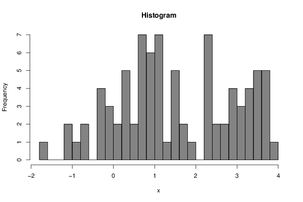
Frequency Table (Histogram)
Bins	Midpoint	Abs. Frequency	Rel. Frequency	Cumul. Rel. Freq.	Density
[-1.8,-1.6[	-1.7	1	0.011905	0.011905	0.059524
[-1.6,-1.4[	-1.5	0	0	0.011905	0
[-1.4,-1.2[	-1.3	0	0	0.011905	0
[-1.2,-1[	-1.1	2	0.02381	0.035714	0.119048
[-1,-0.8[	-0.9	1	0.011905	0.047619	0.059524
[-0.8,-0.6[	-0.7	2	0.02381	0.071429	0.119048
[-0.6,-0.4[	-0.5	0	0	0.071429	0
[-0.4,-0.2[	-0.3	4	0.047619	0.119048	0.238095
[-0.2,0[	-0.1	3	0.035714	0.154762	0.178571
[0,0.2[	0.0999999999999999	2	0.02381	0.178571	0.119048
[0.2,0.4[	0.3	5	0.059524	0.238095	0.297619
[0.4,0.6[	0.5	2	0.02381	0.261905	0.119048
[0.6,0.8[	0.7	7	0.083333	0.345238	0.416667
[0.8,1[	0.9	6	0.071429	0.416667	0.357143
[1,1.2[	1.1	7	0.083333	0.5	0.416667
[1.2,1.4[	1.3	1	0.011905	0.511905	0.059524
[1.4,1.6[	1.5	5	0.059524	0.571429	0.297619
[1.6,1.8[	1.7	2	0.02381	0.595238	0.119048
[1.8,2[	1.9	1	0.011905	0.607143	0.059524
[2,2.2[	2.1	0	0	0.607143	0
[2.2,2.4[	2.3	7	0.083333	0.690476	0.416667
[2.4,2.6[	2.5	2	0.02381	0.714286	0.119048
[2.6,2.8[	2.7	2	0.02381	0.738095	0.119048
[2.8,3[	2.9	4	0.047619	0.785714	0.238095
[3,3.2[	3.1	3	0.035714	0.821429	0.178571
[3.2,3.4[	3.3	4	0.047619	0.869048	0.238095
[3.4,3.6[	3.5	5	0.059524	0.928571	0.297619
[3.6,3.8[	3.7	5	0.059524	0.988095	0.297619
[3.8,4]	3.9	1	0.011905	1	0.059524

\begin{tabular}{lllllllll}
\hline
Frequency Table (Histogram) \tabularnewline
Bins & Midpoint & Abs. Frequency & Rel. Frequency & Cumul. Rel. Freq. & Density \tabularnewline
[-1.8,-1.6[ & -1.7 & 1 & 0.011905 & 0.011905 & 0.059524 \tabularnewline
[-1.6,-1.4[ & -1.5 & 0 & 0 & 0.011905 & 0 \tabularnewline
[-1.4,-1.2[ & -1.3 & 0 & 0 & 0.011905 & 0 \tabularnewline
[-1.2,-1[ & -1.1 & 2 & 0.02381 & 0.035714 & 0.119048 \tabularnewline
[-1,-0.8[ & -0.9 & 1 & 0.011905 & 0.047619 & 0.059524 \tabularnewline
[-0.8,-0.6[ & -0.7 & 2 & 0.02381 & 0.071429 & 0.119048 \tabularnewline
[-0.6,-0.4[ & -0.5 & 0 & 0 & 0.071429 & 0 \tabularnewline
[-0.4,-0.2[ & -0.3 & 4 & 0.047619 & 0.119048 & 0.238095 \tabularnewline
[-0.2,0[ & -0.1 & 3 & 0.035714 & 0.154762 & 0.178571 \tabularnewline
[0,0.2[ & 0.0999999999999999 & 2 & 0.02381 & 0.178571 & 0.119048 \tabularnewline
[0.2,0.4[ & 0.3 & 5 & 0.059524 & 0.238095 & 0.297619 \tabularnewline
[0.4,0.6[ & 0.5 & 2 & 0.02381 & 0.261905 & 0.119048 \tabularnewline
[0.6,0.8[ & 0.7 & 7 & 0.083333 & 0.345238 & 0.416667 \tabularnewline
[0.8,1[ & 0.9 & 6 & 0.071429 & 0.416667 & 0.357143 \tabularnewline
[1,1.2[ & 1.1 & 7 & 0.083333 & 0.5 & 0.416667 \tabularnewline
[1.2,1.4[ & 1.3 & 1 & 0.011905 & 0.511905 & 0.059524 \tabularnewline
[1.4,1.6[ & 1.5 & 5 & 0.059524 & 0.571429 & 0.297619 \tabularnewline
[1.6,1.8[ & 1.7 & 2 & 0.02381 & 0.595238 & 0.119048 \tabularnewline
[1.8,2[ & 1.9 & 1 & 0.011905 & 0.607143 & 0.059524 \tabularnewline
[2,2.2[ & 2.1 & 0 & 0 & 0.607143 & 0 \tabularnewline
[2.2,2.4[ & 2.3 & 7 & 0.083333 & 0.690476 & 0.416667 \tabularnewline
[2.4,2.6[ & 2.5 & 2 & 0.02381 & 0.714286 & 0.119048 \tabularnewline
[2.6,2.8[ & 2.7 & 2 & 0.02381 & 0.738095 & 0.119048 \tabularnewline
[2.8,3[ & 2.9 & 4 & 0.047619 & 0.785714 & 0.238095 \tabularnewline
[3,3.2[ & 3.1 & 3 & 0.035714 & 0.821429 & 0.178571 \tabularnewline
[3.2,3.4[ & 3.3 & 4 & 0.047619 & 0.869048 & 0.238095 \tabularnewline
[3.4,3.6[ & 3.5 & 5 & 0.059524 & 0.928571 & 0.297619 \tabularnewline
[3.6,3.8[ & 3.7 & 5 & 0.059524 & 0.988095 & 0.297619 \tabularnewline
[3.8,4] & 3.9 & 1 & 0.011905 & 1 & 0.059524 \tabularnewline
\hline
\end{tabular}
%Source: https://freestatistics.org/blog/index.php?pk=&T=1

[TABLE]
[ROW][C]Frequency Table (Histogram)[/C][/ROW]
[ROW][C]Bins[/C][C]Midpoint[/C][C]Abs. Frequency[/C][C]Rel. Frequency[/C][C]Cumul. Rel. Freq.[/C][C]Density[/C][/ROW]
[ROW][C][-1.8,-1.6[[/C][C]-1.7[/C][C]1[/C][C]0.011905[/C][C]0.011905[/C][C]0.059524[/C][/ROW]
[ROW][C][-1.6,-1.4[[/C][C]-1.5[/C][C]0[/C][C]0[/C][C]0.011905[/C][C]0[/C][/ROW]
[ROW][C][-1.4,-1.2[[/C][C]-1.3[/C][C]0[/C][C]0[/C][C]0.011905[/C][C]0[/C][/ROW]
[ROW][C][-1.2,-1[[/C][C]-1.1[/C][C]2[/C][C]0.02381[/C][C]0.035714[/C][C]0.119048[/C][/ROW]
[ROW][C][-1,-0.8[[/C][C]-0.9[/C][C]1[/C][C]0.011905[/C][C]0.047619[/C][C]0.059524[/C][/ROW]
[ROW][C][-0.8,-0.6[[/C][C]-0.7[/C][C]2[/C][C]0.02381[/C][C]0.071429[/C][C]0.119048[/C][/ROW]
[ROW][C][-0.6,-0.4[[/C][C]-0.5[/C][C]0[/C][C]0[/C][C]0.071429[/C][C]0[/C][/ROW]
[ROW][C][-0.4,-0.2[[/C][C]-0.3[/C][C]4[/C][C]0.047619[/C][C]0.119048[/C][C]0.238095[/C][/ROW]
[ROW][C][-0.2,0[[/C][C]-0.1[/C][C]3[/C][C]0.035714[/C][C]0.154762[/C][C]0.178571[/C][/ROW]
[ROW][C][0,0.2[[/C][C]0.0999999999999999[/C][C]2[/C][C]0.02381[/C][C]0.178571[/C][C]0.119048[/C][/ROW]
[ROW][C][0.2,0.4[[/C][C]0.3[/C][C]5[/C][C]0.059524[/C][C]0.238095[/C][C]0.297619[/C][/ROW]
[ROW][C][0.4,0.6[[/C][C]0.5[/C][C]2[/C][C]0.02381[/C][C]0.261905[/C][C]0.119048[/C][/ROW]
[ROW][C][0.6,0.8[[/C][C]0.7[/C][C]7[/C][C]0.083333[/C][C]0.345238[/C][C]0.416667[/C][/ROW]
[ROW][C][0.8,1[[/C][C]0.9[/C][C]6[/C][C]0.071429[/C][C]0.416667[/C][C]0.357143[/C][/ROW]
[ROW][C][1,1.2[[/C][C]1.1[/C][C]7[/C][C]0.083333[/C][C]0.5[/C][C]0.416667[/C][/ROW]
[ROW][C][1.2,1.4[[/C][C]1.3[/C][C]1[/C][C]0.011905[/C][C]0.511905[/C][C]0.059524[/C][/ROW]
[ROW][C][1.4,1.6[[/C][C]1.5[/C][C]5[/C][C]0.059524[/C][C]0.571429[/C][C]0.297619[/C][/ROW]
[ROW][C][1.6,1.8[[/C][C]1.7[/C][C]2[/C][C]0.02381[/C][C]0.595238[/C][C]0.119048[/C][/ROW]
[ROW][C][1.8,2[[/C][C]1.9[/C][C]1[/C][C]0.011905[/C][C]0.607143[/C][C]0.059524[/C][/ROW]
[ROW][C][2,2.2[[/C][C]2.1[/C][C]0[/C][C]0[/C][C]0.607143[/C][C]0[/C][/ROW]
[ROW][C][2.2,2.4[[/C][C]2.3[/C][C]7[/C][C]0.083333[/C][C]0.690476[/C][C]0.416667[/C][/ROW]
[ROW][C][2.4,2.6[[/C][C]2.5[/C][C]2[/C][C]0.02381[/C][C]0.714286[/C][C]0.119048[/C][/ROW]
[ROW][C][2.6,2.8[[/C][C]2.7[/C][C]2[/C][C]0.02381[/C][C]0.738095[/C][C]0.119048[/C][/ROW]
[ROW][C][2.8,3[[/C][C]2.9[/C][C]4[/C][C]0.047619[/C][C]0.785714[/C][C]0.238095[/C][/ROW]
[ROW][C][3,3.2[[/C][C]3.1[/C][C]3[/C][C]0.035714[/C][C]0.821429[/C][C]0.178571[/C][/ROW]
[ROW][C][3.2,3.4[[/C][C]3.3[/C][C]4[/C][C]0.047619[/C][C]0.869048[/C][C]0.238095[/C][/ROW]
[ROW][C][3.4,3.6[[/C][C]3.5[/C][C]5[/C][C]0.059524[/C][C]0.928571[/C][C]0.297619[/C][/ROW]
[ROW][C][3.6,3.8[[/C][C]3.7[/C][C]5[/C][C]0.059524[/C][C]0.988095[/C][C]0.297619[/C][/ROW]
[ROW][C][3.8,4][/C][C]3.9[/C][C]1[/C][C]0.011905[/C][C]1[/C][C]0.059524[/C][/ROW]
[/TABLE]
Source: https://freestatistics.org/blog/index.php?pk=&T=1

Globally Unique Identifier (entire table): ba.freestatistics.org/blog/index.php?pk=&T=1

As an alternative you can also use a QR Code:

The GUIDs for individual cells are displayed in the table below:

Frequency Table (Histogram)
Bins	Midpoint	Abs. Frequency	Rel. Frequency	Cumul. Rel. Freq.	Density
[-1.8,-1.6[	-1.7	1	0.011905	0.011905	0.059524
[-1.6,-1.4[	-1.5	0	0	0.011905	0
[-1.4,-1.2[	-1.3	0	0	0.011905	0
[-1.2,-1[	-1.1	2	0.02381	0.035714	0.119048
[-1,-0.8[	-0.9	1	0.011905	0.047619	0.059524
[-0.8,-0.6[	-0.7	2	0.02381	0.071429	0.119048
[-0.6,-0.4[	-0.5	0	0	0.071429	0
[-0.4,-0.2[	-0.3	4	0.047619	0.119048	0.238095
[-0.2,0[	-0.1	3	0.035714	0.154762	0.178571
[0,0.2[	0.0999999999999999	2	0.02381	0.178571	0.119048
[0.2,0.4[	0.3	5	0.059524	0.238095	0.297619
[0.4,0.6[	0.5	2	0.02381	0.261905	0.119048
[0.6,0.8[	0.7	7	0.083333	0.345238	0.416667
[0.8,1[	0.9	6	0.071429	0.416667	0.357143
[1,1.2[	1.1	7	0.083333	0.5	0.416667
[1.2,1.4[	1.3	1	0.011905	0.511905	0.059524
[1.4,1.6[	1.5	5	0.059524	0.571429	0.297619
[1.6,1.8[	1.7	2	0.02381	0.595238	0.119048
[1.8,2[	1.9	1	0.011905	0.607143	0.059524
[2,2.2[	2.1	0	0	0.607143	0
[2.2,2.4[	2.3	7	0.083333	0.690476	0.416667
[2.4,2.6[	2.5	2	0.02381	0.714286	0.119048
[2.6,2.8[	2.7	2	0.02381	0.738095	0.119048
[2.8,3[	2.9	4	0.047619	0.785714	0.238095
[3,3.2[	3.1	3	0.035714	0.821429	0.178571
[3.2,3.4[	3.3	4	0.047619	0.869048	0.238095
[3.4,3.6[	3.5	5	0.059524	0.928571	0.297619
[3.6,3.8[	3.7	5	0.059524	0.988095	0.297619
[3.8,4]	3.9	1	0.011905	1	0.059524

Figure 1

PNG link

Postscript link

PDF link

Parameters (Session):

par1 = 24 ; par2 = grey ; par3 = FALSE ; par4 = Unknown ;

Parameters (R input):

par1 = 24 ; par2 = grey ; par3 = FALSE ; par4 = Unknown ;

R code (references can be found in the software module):

par4 <- 'Unknown'
par3 <- 'FALSE'
par2 <- 'grey'
par1 <- '11'
par1 <- as.numeric(par1)
if (par3 == 'TRUE') par3 <- TRUE
if (par3 == 'FALSE') par3 <- FALSE
if (par4 == 'Unknown') par1 <- as.numeric(par1)
if (par4 == 'Interval/Ratio') par1 <- as.numeric(par1)
if (par4 == '3-point Likert') par1 <- c(1:3 - 0.5, 3.5)
if (par4 == '4-point Likert') par1 <- c(1:4 - 0.5, 4.5)
if (par4 == '5-point Likert') par1 <- c(1:5 - 0.5, 5.5)
if (par4 == '6-point Likert') par1 <- c(1:6 - 0.5, 6.5)
if (par4 == '7-point Likert') par1 <- c(1:7 - 0.5, 7.5)
if (par4 == '8-point Likert') par1 <- c(1:8 - 0.5, 8.5)
if (par4 == '9-point Likert') par1 <- c(1:9 - 0.5, 9.5)
if (par4 == '10-point Likert') par1 <- c(1:10 - 0.5, 10.5)
bitmap(file='test1.png')
if(is.numeric(x[1])) {
if (is.na(par1)) {
myhist<-hist(x,col=par2,main=main,xlab=xlab,right=par3)
} else {
if (par1 < 0) par1 <- 3
if (par1 > 50) par1 <- 50
myhist<-hist(x,breaks=par1,col=par2,main=main,xlab=xlab,right=par3)
}
} else {
barplot(mytab <- sort(table(x),T),col=par2,main='Frequency Plot',xlab=xlab,ylab='Absolute Frequency')
}
dev.off()
if(is.numeric(x[1])) {
myhist
n <- length(x)
load(file='createtable')
a<-table.start()
a<-table.row.start(a)
a<-table.element(a,hyperlink('histogram.htm','Frequency Table (Histogram)',''),6,TRUE)
a<-table.row.end(a)
a<-table.row.start(a)
a<-table.element(a,'Bins',header=TRUE)
a<-table.element(a,'Midpoint',header=TRUE)
a<-table.element(a,'Abs. Frequency',header=TRUE)
a<-table.element(a,'Rel. Frequency',header=TRUE)
a<-table.element(a,'Cumul. Rel. Freq.',header=TRUE)
a<-table.element(a,'Density',header=TRUE)
a<-table.row.end(a)
crf <- 0
if (par3 == FALSE) mybracket <- '[' else mybracket <- ']'
mynumrows <- (length(myhist$breaks)-1)
for (i in 1:mynumrows) {
a<-table.row.start(a)
if (i == 1)
dum <- paste('[',myhist$breaks[i],sep='')
else
dum <- paste(mybracket,myhist$breaks[i],sep='')
dum <- paste(dum,myhist$breaks[i+1],sep=',')
if (i==mynumrows)
dum <- paste(dum,']',sep='')
else
dum <- paste(dum,mybracket,sep='')
a<-table.element(a,dum,header=TRUE)
a<-table.element(a,myhist$mids[i])
a<-table.element(a,myhist$counts[i])
rf <- myhist$counts[i]/n
crf <- crf + rf
a<-table.element(a,round(rf,6))
a<-table.element(a,round(crf,6))
a<-table.element(a,round(myhist$density[i],6))
a<-table.row.end(a)
}
a<-table.end(a)
table.save(a,file='mytable.tab')
} else {
mytab
reltab <- mytab / sum(mytab)
n <- length(mytab)
load(file='createtable')
a<-table.start()
a<-table.row.start(a)
a<-table.element(a,'Frequency Table (Categorical Data)',3,TRUE)
a<-table.row.end(a)
a<-table.row.start(a)
a<-table.element(a,'Category',header=TRUE)
a<-table.element(a,'Abs. Frequency',header=TRUE)
a<-table.element(a,'Rel. Frequency',header=TRUE)
a<-table.row.end(a)
for (i in 1:n) {
a<-table.row.start(a)
a<-table.element(a,labels(mytab)$x[i],header=TRUE)
a<-table.element(a,mytab[i])
a<-table.element(a,round(reltab[i],4))
a<-table.row.end(a)
}
a<-table.end(a)
table.save(a,file='mytable1.tab')
}

Free Statistics

Description of Statistical Computation

Tree of Dependent Computations

Dataset

Tables (Output of Computation)

Figures (Output of Computation)

Input Parameters & R Code