Repository of Reproducible Computations

Free Statistics

of Irreproducible Research!

Author's title

Author

*The author of this computation has been verified*

R Software Module

rwasp_fitdistrnorm.wasp

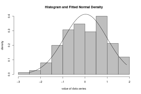
Title produced by software

ML Fitting and QQ Plot- Normal Distribution

Date of computation

Fri, 07 Oct 2016 14:03:49 +0200

Cite this page as follows

Statistical Computations at FreeStatistics.org, Office for Research Development and Education, URL https://freestatistics.org/blog/index.php?v=date/2016/Oct/07/t14758418751ul6swiqf6pbzyt.htm/, Retrieved Tue, 21 May 2024 08:32:24 +0000

Statistical Computations at FreeStatistics.org, Office for Research Development and Education, URL https://freestatistics.org/blog/index.php?pk=296589, Retrieved Tue, 21 May 2024 08:32:24 +0000

QR Codes:

Paste this QR Code to cite your computation.

Original text written by user:

IsPrivate?

No (this computation is public)

User-defined keywords

Estimated Impact

Family? (F = Feedback message, R = changed R code, M = changed R Module, P = changed Parameters, D = changed Data)

-       [ML Fitting and QQ Plot- Normal Distribution] [] [2016-10-07 12:03:49] [24da340c2401d75222b6137c0718139b] [Current]

Feedback Forum

Post a new message

Dataseries X:

Download CSV

Histogram

Boxplots

-0.6380267209
-0.7130878669
1.210173204
-0.8274471141
-1.683341053
1.815686454
-1.221736821
-0.2079142092
1.296409394
-0.874202214
0.3448860652
-2.103751252
-0.3891857369
-0.2173946398
-1.21306628
1.123516837
-0.2066682079
-0.9296374988
1.506741283
-1.587869318
-0.9244683654
0.6500533372
0.8985177496
0.9001210222
0.3457131589
0.2016047946
-0.7008489243
-0.1902921007
-1.408101363
-1.949526149
-0.5766102705
-0.6839247166
1.829201299
-0.2213911469
1.283397742
1.400520404
0.5115686914
-0.1802131906
-2.40731452
-1.312021991
-0.5720994202
1.039325268
-1.345584488
0.2689200206
1.082542272
0.2981690492
-1.265917015
0.5056298483
0.5601528534
-0.9986475794
-0.08342845629
-0.1771482629
-0.1250518943
-0.3691641498
-1.552416162
-2.5171847
0.8043189723
1.26271789
0.5594472849
0.3446348765
1.206824457
-0.9311776985
0.7812945852
1.608083997
1.824559934
0.802659615
-0.266380461
0.5417444992
-0.430099602
0.2697643997
1.407207767
0.195531565
1.296618308
-0.2175930912
0.9264420387
1.097592533
-0.9446228886
0.5986802506
0.7969833798
-0.06441851249
0.8335990687
-1.654037896
0.6378263328
1.222308862
0.7797089508
0.4287515842
-0.6022700332
0.9457657271
-0.08824862077
1.420881416
0.05602326979
1.203523109
0.3103849063
-0.5578953708
0.8077859267
-0.178493557
-0.2037506217
-0.4809433368
-0.2665958765
0.9571451596
0.09170975642
-0.06940811892
0.9525008869
-1.313103108
-0.5330262578
0.5374959953
-1.737758013
-0.4218529159
-1.129414661
0.09657264894
-0.7399833273
-0.7545169253
0.5442927543
0.5591055083
-1.049507087
-0.1086560926
0.1222916579
-0.6463050127
-1.162951217
-1.168955456
0.2148435839
-0.3465296515
0.4975772644
0.002175190273
-0.5237315173
0.6276764365
0.6446675829
0.4583759498
-0.8426863463
0.677635937
1.670160644
-1.15251396
1.141896276
1.657085746
0.6740795268
1.874068204
-0.531778186
0.07688941806
-1.022064442
-1.253691608
0.334277361
0.2941236161
-0.8775914703
1.607289785
-0.4123004976
0.6855406
0.3494025727
-0.04935754691
0.7000176686
-1.194595567

Summary of computational transaction
Raw Input	view raw input (R code)
Raw Output	view raw output of R engine
Computing time	3 seconds
R Server	Big Analytics Cloud Computing Center

\begin{tabular}{lllllllll}
\hline
Summary of computational transaction \tabularnewline
Raw Input view raw input (R code)  \tabularnewline
Raw Outputview raw output of R engine  \tabularnewline
Computing time3 seconds \tabularnewline
R ServerBig Analytics Cloud Computing Center \tabularnewline
\hline
\end{tabular}
%Source: https://freestatistics.org/blog/index.php?pk=296589&T=0

[TABLE]
[ROW]

Summary of computational transaction[/C][/ROW] [ROW]

Raw Input[/C]

view raw input (R code) [/C][/ROW] [ROW]

Raw Output[/C]

view raw output of R engine [/C][/ROW] [ROW]

Computing time[/C]

3 seconds[/C][/ROW] [ROW]

R Server[/C]

Big Analytics Cloud Computing Center[/C][/ROW] [/TABLE] Source: https://freestatistics.org/blog/index.php?pk=296589&T=0

Globally Unique Identifier (entire table): ba.freestatistics.org/blog/index.php?pk=296589&T=0

As an alternative you can also use a QR Code:

The GUIDs for individual cells are displayed in the table below:

Summary of computational transaction
Raw Input	view raw input (R code)
Raw Output	view raw output of R engine
Computing time	3 seconds
R Server	Big Analytics Cloud Computing Center

Parameter	Estimated Value	Standard Deviation
mean	0.0252661575613533	0.0787212302803534
standard deviation	0.96413423055499	0.0556643157545856

\begin{tabular}{lllllllll}
\hline
Parameter & Estimated Value & Standard Deviation \tabularnewline
mean & 0.0252661575613533 & 0.0787212302803534 \tabularnewline
standard deviation & 0.96413423055499 & 0.0556643157545856 \tabularnewline
\hline
\end{tabular}
%Source: https://freestatistics.org/blog/index.php?pk=296589&T=1

[TABLE]
[ROW][C]Parameter[/C][C]Estimated Value[/C][C]Standard Deviation[/C][/ROW]
[ROW][C]mean[/C][C]0.0252661575613533[/C][C]0.0787212302803534[/C][/ROW]
[ROW][C]standard deviation[/C][C]0.96413423055499[/C][C]0.0556643157545856[/C][/ROW]
[/TABLE]
Source: https://freestatistics.org/blog/index.php?pk=296589&T=1

Globally Unique Identifier (entire table): ba.freestatistics.org/blog/index.php?pk=296589&T=1

As an alternative you can also use a QR Code:

The GUIDs for individual cells are displayed in the table below:

Parameter	Estimated Value	Standard Deviation
mean	0.0252661575613533	0.0787212302803534
standard deviation	0.96413423055499	0.0556643157545856

Figure 1

PNG link

Postscript link

PDF link

Figure 2

PNG link

Postscript link

PDF link

Parameters (Session):

par1 = 8 ; par2 = 0 ;

Parameters (R input):

par1 = 8 ; par2 = 0 ;

R code (references can be found in the software module):

library(MASS)
library(car)
par1 <- as.numeric(par1)
if (par2 == '0') par2 = 'Sturges' else par2 <- as.numeric(par2)
x <- as.ts(x) #otherwise the fitdistr function does not work properly
r <- fitdistr(x,'normal')
print(r)
bitmap(file='test1.png')
myhist<-hist(x,col=par1,breaks=par2,main=main,ylab=ylab,xlab=xlab,freq=F)
curve(1/(r$estimate[2]*sqrt(2*pi))*exp(-1/2*((x-r$estimate[1])/r$estimate[2])^2),min(x),max(x),add=T)
dev.off()
bitmap(file='test3.png')
qqPlot(x,dist='norm',main='QQ plot (Normal) with confidence intervals')
grid()
dev.off()
load(file='createtable')
a<-table.start()
a<-table.row.start(a)
a<-table.element(a,'Parameter',1,TRUE)
a<-table.element(a,'Estimated Value',1,TRUE)
a<-table.element(a,'Standard Deviation',1,TRUE)
a<-table.row.end(a)
a<-table.row.start(a)
a<-table.element(a,'mean',header=TRUE)
a<-table.element(a,r$estimate[1])
a<-table.element(a,r$sd[1])
a<-table.row.end(a)
a<-table.row.start(a)
a<-table.element(a,'standard deviation',header=TRUE)
a<-table.element(a,r$estimate[2])
a<-table.element(a,r$sd[2])
a<-table.row.end(a)
a<-table.end(a)
table.save(a,file='mytable.tab')

Free Statistics

Description of Statistical Computation

Tree of Dependent Computations

Dataset

Tables (Output of Computation)

Figures (Output of Computation)

Input Parameters & R Code