Repository of Reproducible Computations

Free Statistics

of Irreproducible Research!

Author's title

Author

*Unverified author*

R Software Module

rwasp_decompose.wasp

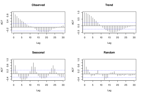
Title produced by software

Classical Decomposition

Date of computation

Mon, 28 Nov 2016 14:17:10 +0000

Cite this page as follows

Statistical Computations at FreeStatistics.org, Office for Research Development and Education, URL https://freestatistics.org/blog/index.php?v=date/2016/Nov/28/t1480342662n8r4lfxfihnhhsx.htm/, Retrieved Sun, 19 May 2024 04:17:39 +0200

Statistical Computations at FreeStatistics.org, Office for Research Development and Education, URL https://freestatistics.org/blog/index.php?pk=, Retrieved Sun, 19 May 2024 04:17:39 +0200

QR Codes:

Paste this QR Code to cite your computation.

Original text written by user:

IsPrivate?

No (this computation is public)

User-defined keywords

Estimated Impact

Dataseries X:

Download CSV

Histogram

Boxplots

Summary of computational transaction
Raw Input	view raw input (R code)
Raw Output	view raw output of R engine
Computing time	2 seconds
R Server	'Gwilym Jenkins' @ jenkins.wessa.net

\begin{tabular}{lllllllll}
\hline
Summary of computational transaction \tabularnewline
Raw Input & view raw input (R code)  \tabularnewline
Raw Output & view raw output of R engine  \tabularnewline
Computing time & 2 seconds \tabularnewline
R Server & 'Gwilym Jenkins' @ jenkins.wessa.net \tabularnewline
\hline
\end{tabular}
%Source: https://freestatistics.org/blog/index.php?pk=&T=0

[TABLE]
[ROW][C]Summary of computational transaction[/C][/ROW]
[ROW][C]Raw Input[/C][C]view raw input (R code) [/C][/ROW]
[ROW][C]Raw Output[/C][C]view raw output of R engine [/C][/ROW]
[ROW][C]Computing time[/C][C]2 seconds[/C][/ROW]
[ROW][C]R Server[/C][C]'Gwilym Jenkins' @ jenkins.wessa.net[/C][/ROW]
[/TABLE]
Source: https://freestatistics.org/blog/index.php?pk=&T=0

Globally Unique Identifier (entire table): ba.freestatistics.org/blog/index.php?pk=&T=0

As an alternative you can also use a QR Code:

The GUIDs for individual cells are displayed in the table below:

Summary of computational transaction
Raw Input	view raw input (R code)
Raw Output	view raw output of R engine
Computing time	2 seconds
R Server	'Gwilym Jenkins' @ jenkins.wessa.net

Classical Decomposition by Moving Averages
t	Observations	Fit	Trend	Seasonal	Random
1	91.19	NA	NA	-1.67599	NA
2	95.06	NA	NA	0.309635	NA
3	95.61	NA	NA	0.985469	NA
4	97.13	NA	NA	2.53974	NA
5	95.44	NA	NA	2.16703	NA
6	94.65	NA	NA	1.55307	NA
7	93.46	92.7389	93.7154	-0.97651	0.721094
8	92.19	92.2371	93.6658	-1.4287	-0.0471354
9	93.49	93.6586	93.5617	0.0969271	-0.168594
10	92.73	93.0181	93.49	-0.471927	-0.288073
11	91.4	91.5726	93.495	-1.92245	-0.172552
12	92.16	92.4533	93.6296	-1.1763	-0.293281
13	91.34	92.1028	93.7788	-1.67599	-0.76276
14	93.72	94.2196	93.91	0.309635	-0.499635
15	94.45	95.1617	94.1763	0.985469	-0.711719
16	96.57	97.1652	94.6254	2.53974	-0.595156
17	96.12	97.3149	95.1479	2.16703	-1.19495
18	97.2	97.3056	95.7525	1.55307	-0.105573
19	94.49	95.4827	96.4592	-0.97651	-0.992656
20	94.31	95.7692	97.1979	-1.4287	-1.45922
21	97.76	98.034	97.9371	0.0969271	-0.27401
22	99.24	98.1843	98.6562	-0.471927	1.05568
23	97.43	97.5601	99.4825	-1.92245	-0.130052
24	100.64	99.1249	100.301	-1.1763	1.51505
25	99.82	99.3123	100.988	-1.67599	0.507656
26	102.97	101.916	101.607	0.309635	1.0537
27	102.94	103.049	102.064	0.985469	-0.109219
28	105.34	104.808	102.268	2.53974	0.532344
29	107.18	104.447	102.28	2.16703	2.73255
30	105.79	103.657	102.104	1.55307	2.13318
31	102.39	100.886	101.862	-0.97651	1.50401
32	101.25	100.15	101.578	-1.4287	1.10036
33	101.79	101.411	101.314	0.0969271	0.379323
34	100.11	100.623	101.095	-0.471927	-0.512656
35	96.86	98.7042	100.627	-1.92245	-1.84422
36	96.97	98.8424	100.019	-1.1763	-1.87245
37	97.7	97.7498	99.4258	-1.67599	-0.0498437
38	98.27	99.2238	98.9142	0.309635	-0.953802
39	101.29	99.5021	98.5167	0.985469	1.78786
40	101.73	100.704	98.1642	2.53974	1.02609
41	99.56	100.176	98.0087	2.16703	-0.615781
42	98.82	99.5456	97.9925	1.55307	-0.725573
43	95.13	96.9081	97.8846	-0.97651	-1.77807
44	96.23	96.3696	97.7983	-1.4287	-0.139635
45	97.27	97.7523	97.6554	0.0969271	-0.482344
46	96.17	96.9706	97.4425	-0.471927	-0.800573
47	97.07	95.4688	97.3912	-1.92245	1.6012
48	96.37	96.2649	97.4412	-1.1763	0.105052
49	95.71	95.9507	97.6267	-1.67599	-0.240677
50	98.19	98.3359	98.0262	0.309635	-0.145885
51	97.94	99.4526	98.4671	0.985469	-1.51255
52	99.97	101.479	98.9392	2.53974	-1.50891
53	100.09	101.557	99.3904	2.16703	-1.46745
54	99.49	101.338	99.7846	1.55307	-1.84766
55	98.91	NA	NA	-0.97651	NA
56	102.04	NA	NA	-1.4287	NA
57	102.04	NA	NA	0.0969271	NA
58	102.73	NA	NA	-0.471927	NA
59	101.34	NA	NA	-1.92245	NA
60	101.56	NA	NA	-1.1763	NA

\begin{tabular}{lllllllll}
\hline
Classical Decomposition by Moving Averages \tabularnewline
t & Observations & Fit & Trend & Seasonal & Random \tabularnewline
1 & 91.19 & NA & NA & -1.67599 & NA \tabularnewline
2 & 95.06 & NA & NA & 0.309635 & NA \tabularnewline
3 & 95.61 & NA & NA & 0.985469 & NA \tabularnewline
4 & 97.13 & NA & NA & 2.53974 & NA \tabularnewline
5 & 95.44 & NA & NA & 2.16703 & NA \tabularnewline
6 & 94.65 & NA & NA & 1.55307 & NA \tabularnewline
7 & 93.46 & 92.7389 & 93.7154 & -0.97651 & 0.721094 \tabularnewline
8 & 92.19 & 92.2371 & 93.6658 & -1.4287 & -0.0471354 \tabularnewline
9 & 93.49 & 93.6586 & 93.5617 & 0.0969271 & -0.168594 \tabularnewline
10 & 92.73 & 93.0181 & 93.49 & -0.471927 & -0.288073 \tabularnewline
11 & 91.4 & 91.5726 & 93.495 & -1.92245 & -0.172552 \tabularnewline
12 & 92.16 & 92.4533 & 93.6296 & -1.1763 & -0.293281 \tabularnewline
13 & 91.34 & 92.1028 & 93.7788 & -1.67599 & -0.76276 \tabularnewline
14 & 93.72 & 94.2196 & 93.91 & 0.309635 & -0.499635 \tabularnewline
15 & 94.45 & 95.1617 & 94.1763 & 0.985469 & -0.711719 \tabularnewline
16 & 96.57 & 97.1652 & 94.6254 & 2.53974 & -0.595156 \tabularnewline
17 & 96.12 & 97.3149 & 95.1479 & 2.16703 & -1.19495 \tabularnewline
18 & 97.2 & 97.3056 & 95.7525 & 1.55307 & -0.105573 \tabularnewline
19 & 94.49 & 95.4827 & 96.4592 & -0.97651 & -0.992656 \tabularnewline
20 & 94.31 & 95.7692 & 97.1979 & -1.4287 & -1.45922 \tabularnewline
21 & 97.76 & 98.034 & 97.9371 & 0.0969271 & -0.27401 \tabularnewline
22 & 99.24 & 98.1843 & 98.6562 & -0.471927 & 1.05568 \tabularnewline
23 & 97.43 & 97.5601 & 99.4825 & -1.92245 & -0.130052 \tabularnewline
24 & 100.64 & 99.1249 & 100.301 & -1.1763 & 1.51505 \tabularnewline
25 & 99.82 & 99.3123 & 100.988 & -1.67599 & 0.507656 \tabularnewline
26 & 102.97 & 101.916 & 101.607 & 0.309635 & 1.0537 \tabularnewline
27 & 102.94 & 103.049 & 102.064 & 0.985469 & -0.109219 \tabularnewline
28 & 105.34 & 104.808 & 102.268 & 2.53974 & 0.532344 \tabularnewline
29 & 107.18 & 104.447 & 102.28 & 2.16703 & 2.73255 \tabularnewline
30 & 105.79 & 103.657 & 102.104 & 1.55307 & 2.13318 \tabularnewline
31 & 102.39 & 100.886 & 101.862 & -0.97651 & 1.50401 \tabularnewline
32 & 101.25 & 100.15 & 101.578 & -1.4287 & 1.10036 \tabularnewline
33 & 101.79 & 101.411 & 101.314 & 0.0969271 & 0.379323 \tabularnewline
34 & 100.11 & 100.623 & 101.095 & -0.471927 & -0.512656 \tabularnewline
35 & 96.86 & 98.7042 & 100.627 & -1.92245 & -1.84422 \tabularnewline
36 & 96.97 & 98.8424 & 100.019 & -1.1763 & -1.87245 \tabularnewline
37 & 97.7 & 97.7498 & 99.4258 & -1.67599 & -0.0498437 \tabularnewline
38 & 98.27 & 99.2238 & 98.9142 & 0.309635 & -0.953802 \tabularnewline
39 & 101.29 & 99.5021 & 98.5167 & 0.985469 & 1.78786 \tabularnewline
40 & 101.73 & 100.704 & 98.1642 & 2.53974 & 1.02609 \tabularnewline
41 & 99.56 & 100.176 & 98.0087 & 2.16703 & -0.615781 \tabularnewline
42 & 98.82 & 99.5456 & 97.9925 & 1.55307 & -0.725573 \tabularnewline
43 & 95.13 & 96.9081 & 97.8846 & -0.97651 & -1.77807 \tabularnewline
44 & 96.23 & 96.3696 & 97.7983 & -1.4287 & -0.139635 \tabularnewline
45 & 97.27 & 97.7523 & 97.6554 & 0.0969271 & -0.482344 \tabularnewline
46 & 96.17 & 96.9706 & 97.4425 & -0.471927 & -0.800573 \tabularnewline
47 & 97.07 & 95.4688 & 97.3912 & -1.92245 & 1.6012 \tabularnewline
48 & 96.37 & 96.2649 & 97.4412 & -1.1763 & 0.105052 \tabularnewline
49 & 95.71 & 95.9507 & 97.6267 & -1.67599 & -0.240677 \tabularnewline
50 & 98.19 & 98.3359 & 98.0262 & 0.309635 & -0.145885 \tabularnewline
51 & 97.94 & 99.4526 & 98.4671 & 0.985469 & -1.51255 \tabularnewline
52 & 99.97 & 101.479 & 98.9392 & 2.53974 & -1.50891 \tabularnewline
53 & 100.09 & 101.557 & 99.3904 & 2.16703 & -1.46745 \tabularnewline
54 & 99.49 & 101.338 & 99.7846 & 1.55307 & -1.84766 \tabularnewline
55 & 98.91 & NA & NA & -0.97651 & NA \tabularnewline
56 & 102.04 & NA & NA & -1.4287 & NA \tabularnewline
57 & 102.04 & NA & NA & 0.0969271 & NA \tabularnewline
58 & 102.73 & NA & NA & -0.471927 & NA \tabularnewline
59 & 101.34 & NA & NA & -1.92245 & NA \tabularnewline
60 & 101.56 & NA & NA & -1.1763 & NA \tabularnewline
\hline
\end{tabular}
%Source: https://freestatistics.org/blog/index.php?pk=&T=1

[TABLE]
[ROW][C]Classical Decomposition by Moving Averages[/C][/ROW]
[ROW][C]t[/C][C]Observations[/C][C]Fit[/C][C]Trend[/C][C]Seasonal[/C][C]Random[/C][/ROW]
[ROW][C]1[/C][C]91.19[/C][C]NA[/C][C]NA[/C][C]-1.67599[/C][C]NA[/C][/ROW]
[ROW][C]2[/C][C]95.06[/C][C]NA[/C][C]NA[/C][C]0.309635[/C][C]NA[/C][/ROW]
[ROW][C]3[/C][C]95.61[/C][C]NA[/C][C]NA[/C][C]0.985469[/C][C]NA[/C][/ROW]
[ROW][C]4[/C][C]97.13[/C][C]NA[/C][C]NA[/C][C]2.53974[/C][C]NA[/C][/ROW]
[ROW][C]5[/C][C]95.44[/C][C]NA[/C][C]NA[/C][C]2.16703[/C][C]NA[/C][/ROW]
[ROW][C]6[/C][C]94.65[/C][C]NA[/C][C]NA[/C][C]1.55307[/C][C]NA[/C][/ROW]
[ROW][C]7[/C][C]93.46[/C][C]92.7389[/C][C]93.7154[/C][C]-0.97651[/C][C]0.721094[/C][/ROW]
[ROW][C]8[/C][C]92.19[/C][C]92.2371[/C][C]93.6658[/C][C]-1.4287[/C][C]-0.0471354[/C][/ROW]
[ROW][C]9[/C][C]93.49[/C][C]93.6586[/C][C]93.5617[/C][C]0.0969271[/C][C]-0.168594[/C][/ROW]
[ROW][C]10[/C][C]92.73[/C][C]93.0181[/C][C]93.49[/C][C]-0.471927[/C][C]-0.288073[/C][/ROW]
[ROW][C]11[/C][C]91.4[/C][C]91.5726[/C][C]93.495[/C][C]-1.92245[/C][C]-0.172552[/C][/ROW]
[ROW][C]12[/C][C]92.16[/C][C]92.4533[/C][C]93.6296[/C][C]-1.1763[/C][C]-0.293281[/C][/ROW]
[ROW][C]13[/C][C]91.34[/C][C]92.1028[/C][C]93.7788[/C][C]-1.67599[/C][C]-0.76276[/C][/ROW]
[ROW][C]14[/C][C]93.72[/C][C]94.2196[/C][C]93.91[/C][C]0.309635[/C][C]-0.499635[/C][/ROW]
[ROW][C]15[/C][C]94.45[/C][C]95.1617[/C][C]94.1763[/C][C]0.985469[/C][C]-0.711719[/C][/ROW]
[ROW][C]16[/C][C]96.57[/C][C]97.1652[/C][C]94.6254[/C][C]2.53974[/C][C]-0.595156[/C][/ROW]
[ROW][C]17[/C][C]96.12[/C][C]97.3149[/C][C]95.1479[/C][C]2.16703[/C][C]-1.19495[/C][/ROW]
[ROW][C]18[/C][C]97.2[/C][C]97.3056[/C][C]95.7525[/C][C]1.55307[/C][C]-0.105573[/C][/ROW]
[ROW][C]19[/C][C]94.49[/C][C]95.4827[/C][C]96.4592[/C][C]-0.97651[/C][C]-0.992656[/C][/ROW]
[ROW][C]20[/C][C]94.31[/C][C]95.7692[/C][C]97.1979[/C][C]-1.4287[/C][C]-1.45922[/C][/ROW]
[ROW][C]21[/C][C]97.76[/C][C]98.034[/C][C]97.9371[/C][C]0.0969271[/C][C]-0.27401[/C][/ROW]
[ROW][C]22[/C][C]99.24[/C][C]98.1843[/C][C]98.6562[/C][C]-0.471927[/C][C]1.05568[/C][/ROW]
[ROW][C]23[/C][C]97.43[/C][C]97.5601[/C][C]99.4825[/C][C]-1.92245[/C][C]-0.130052[/C][/ROW]
[ROW][C]24[/C][C]100.64[/C][C]99.1249[/C][C]100.301[/C][C]-1.1763[/C][C]1.51505[/C][/ROW]
[ROW][C]25[/C][C]99.82[/C][C]99.3123[/C][C]100.988[/C][C]-1.67599[/C][C]0.507656[/C][/ROW]
[ROW][C]26[/C][C]102.97[/C][C]101.916[/C][C]101.607[/C][C]0.309635[/C][C]1.0537[/C][/ROW]
[ROW][C]27[/C][C]102.94[/C][C]103.049[/C][C]102.064[/C][C]0.985469[/C][C]-0.109219[/C][/ROW]
[ROW][C]28[/C][C]105.34[/C][C]104.808[/C][C]102.268[/C][C]2.53974[/C][C]0.532344[/C][/ROW]
[ROW][C]29[/C][C]107.18[/C][C]104.447[/C][C]102.28[/C][C]2.16703[/C][C]2.73255[/C][/ROW]
[ROW][C]30[/C][C]105.79[/C][C]103.657[/C][C]102.104[/C][C]1.55307[/C][C]2.13318[/C][/ROW]
[ROW][C]31[/C][C]102.39[/C][C]100.886[/C][C]101.862[/C][C]-0.97651[/C][C]1.50401[/C][/ROW]
[ROW][C]32[/C][C]101.25[/C][C]100.15[/C][C]101.578[/C][C]-1.4287[/C][C]1.10036[/C][/ROW]
[ROW][C]33[/C][C]101.79[/C][C]101.411[/C][C]101.314[/C][C]0.0969271[/C][C]0.379323[/C][/ROW]
[ROW][C]34[/C][C]100.11[/C][C]100.623[/C][C]101.095[/C][C]-0.471927[/C][C]-0.512656[/C][/ROW]
[ROW][C]35[/C][C]96.86[/C][C]98.7042[/C][C]100.627[/C][C]-1.92245[/C][C]-1.84422[/C][/ROW]
[ROW][C]36[/C][C]96.97[/C][C]98.8424[/C][C]100.019[/C][C]-1.1763[/C][C]-1.87245[/C][/ROW]
[ROW][C]37[/C][C]97.7[/C][C]97.7498[/C][C]99.4258[/C][C]-1.67599[/C][C]-0.0498437[/C][/ROW]
[ROW][C]38[/C][C]98.27[/C][C]99.2238[/C][C]98.9142[/C][C]0.309635[/C][C]-0.953802[/C][/ROW]
[ROW][C]39[/C][C]101.29[/C][C]99.5021[/C][C]98.5167[/C][C]0.985469[/C][C]1.78786[/C][/ROW]
[ROW][C]40[/C][C]101.73[/C][C]100.704[/C][C]98.1642[/C][C]2.53974[/C][C]1.02609[/C][/ROW]
[ROW][C]41[/C][C]99.56[/C][C]100.176[/C][C]98.0087[/C][C]2.16703[/C][C]-0.615781[/C][/ROW]
[ROW][C]42[/C][C]98.82[/C][C]99.5456[/C][C]97.9925[/C][C]1.55307[/C][C]-0.725573[/C][/ROW]
[ROW][C]43[/C][C]95.13[/C][C]96.9081[/C][C]97.8846[/C][C]-0.97651[/C][C]-1.77807[/C][/ROW]
[ROW][C]44[/C][C]96.23[/C][C]96.3696[/C][C]97.7983[/C][C]-1.4287[/C][C]-0.139635[/C][/ROW]
[ROW][C]45[/C][C]97.27[/C][C]97.7523[/C][C]97.6554[/C][C]0.0969271[/C][C]-0.482344[/C][/ROW]
[ROW][C]46[/C][C]96.17[/C][C]96.9706[/C][C]97.4425[/C][C]-0.471927[/C][C]-0.800573[/C][/ROW]
[ROW][C]47[/C][C]97.07[/C][C]95.4688[/C][C]97.3912[/C][C]-1.92245[/C][C]1.6012[/C][/ROW]
[ROW][C]48[/C][C]96.37[/C][C]96.2649[/C][C]97.4412[/C][C]-1.1763[/C][C]0.105052[/C][/ROW]
[ROW][C]49[/C][C]95.71[/C][C]95.9507[/C][C]97.6267[/C][C]-1.67599[/C][C]-0.240677[/C][/ROW]
[ROW][C]50[/C][C]98.19[/C][C]98.3359[/C][C]98.0262[/C][C]0.309635[/C][C]-0.145885[/C][/ROW]
[ROW][C]51[/C][C]97.94[/C][C]99.4526[/C][C]98.4671[/C][C]0.985469[/C][C]-1.51255[/C][/ROW]
[ROW][C]52[/C][C]99.97[/C][C]101.479[/C][C]98.9392[/C][C]2.53974[/C][C]-1.50891[/C][/ROW]
[ROW][C]53[/C][C]100.09[/C][C]101.557[/C][C]99.3904[/C][C]2.16703[/C][C]-1.46745[/C][/ROW]
[ROW][C]54[/C][C]99.49[/C][C]101.338[/C][C]99.7846[/C][C]1.55307[/C][C]-1.84766[/C][/ROW]
[ROW][C]55[/C][C]98.91[/C][C]NA[/C][C]NA[/C][C]-0.97651[/C][C]NA[/C][/ROW]
[ROW][C]56[/C][C]102.04[/C][C]NA[/C][C]NA[/C][C]-1.4287[/C][C]NA[/C][/ROW]
[ROW][C]57[/C][C]102.04[/C][C]NA[/C][C]NA[/C][C]0.0969271[/C][C]NA[/C][/ROW]
[ROW][C]58[/C][C]102.73[/C][C]NA[/C][C]NA[/C][C]-0.471927[/C][C]NA[/C][/ROW]
[ROW][C]59[/C][C]101.34[/C][C]NA[/C][C]NA[/C][C]-1.92245[/C][C]NA[/C][/ROW]
[ROW][C]60[/C][C]101.56[/C][C]NA[/C][C]NA[/C][C]-1.1763[/C][C]NA[/C][/ROW]
[/TABLE]
Source: https://freestatistics.org/blog/index.php?pk=&T=1

Globally Unique Identifier (entire table): ba.freestatistics.org/blog/index.php?pk=&T=1

As an alternative you can also use a QR Code:

The GUIDs for individual cells are displayed in the table below:

Classical Decomposition by Moving Averages
t	Observations	Fit	Trend	Seasonal	Random
1	91.19	NA	NA	-1.67599	NA
2	95.06	NA	NA	0.309635	NA
3	95.61	NA	NA	0.985469	NA
4	97.13	NA	NA	2.53974	NA
5	95.44	NA	NA	2.16703	NA
6	94.65	NA	NA	1.55307	NA
7	93.46	92.7389	93.7154	-0.97651	0.721094
8	92.19	92.2371	93.6658	-1.4287	-0.0471354
9	93.49	93.6586	93.5617	0.0969271	-0.168594
10	92.73	93.0181	93.49	-0.471927	-0.288073
11	91.4	91.5726	93.495	-1.92245	-0.172552
12	92.16	92.4533	93.6296	-1.1763	-0.293281
13	91.34	92.1028	93.7788	-1.67599	-0.76276
14	93.72	94.2196	93.91	0.309635	-0.499635
15	94.45	95.1617	94.1763	0.985469	-0.711719
16	96.57	97.1652	94.6254	2.53974	-0.595156
17	96.12	97.3149	95.1479	2.16703	-1.19495
18	97.2	97.3056	95.7525	1.55307	-0.105573
19	94.49	95.4827	96.4592	-0.97651	-0.992656
20	94.31	95.7692	97.1979	-1.4287	-1.45922
21	97.76	98.034	97.9371	0.0969271	-0.27401
22	99.24	98.1843	98.6562	-0.471927	1.05568
23	97.43	97.5601	99.4825	-1.92245	-0.130052
24	100.64	99.1249	100.301	-1.1763	1.51505
25	99.82	99.3123	100.988	-1.67599	0.507656
26	102.97	101.916	101.607	0.309635	1.0537
27	102.94	103.049	102.064	0.985469	-0.109219
28	105.34	104.808	102.268	2.53974	0.532344
29	107.18	104.447	102.28	2.16703	2.73255
30	105.79	103.657	102.104	1.55307	2.13318
31	102.39	100.886	101.862	-0.97651	1.50401
32	101.25	100.15	101.578	-1.4287	1.10036
33	101.79	101.411	101.314	0.0969271	0.379323
34	100.11	100.623	101.095	-0.471927	-0.512656
35	96.86	98.7042	100.627	-1.92245	-1.84422
36	96.97	98.8424	100.019	-1.1763	-1.87245
37	97.7	97.7498	99.4258	-1.67599	-0.0498437
38	98.27	99.2238	98.9142	0.309635	-0.953802
39	101.29	99.5021	98.5167	0.985469	1.78786
40	101.73	100.704	98.1642	2.53974	1.02609
41	99.56	100.176	98.0087	2.16703	-0.615781
42	98.82	99.5456	97.9925	1.55307	-0.725573
43	95.13	96.9081	97.8846	-0.97651	-1.77807
44	96.23	96.3696	97.7983	-1.4287	-0.139635
45	97.27	97.7523	97.6554	0.0969271	-0.482344
46	96.17	96.9706	97.4425	-0.471927	-0.800573
47	97.07	95.4688	97.3912	-1.92245	1.6012
48	96.37	96.2649	97.4412	-1.1763	0.105052
49	95.71	95.9507	97.6267	-1.67599	-0.240677
50	98.19	98.3359	98.0262	0.309635	-0.145885
51	97.94	99.4526	98.4671	0.985469	-1.51255
52	99.97	101.479	98.9392	2.53974	-1.50891
53	100.09	101.557	99.3904	2.16703	-1.46745
54	99.49	101.338	99.7846	1.55307	-1.84766
55	98.91	NA	NA	-0.97651	NA
56	102.04	NA	NA	-1.4287	NA
57	102.04	NA	NA	0.0969271	NA
58	102.73	NA	NA	-0.471927	NA
59	101.34	NA	NA	-1.92245	NA
60	101.56	NA	NA	-1.1763	NA

Figure 1

PNG link

Postscript link

PDF link

Figure 2

PNG link

Postscript link

PDF link

Figure 3

PNG link

Postscript link

PDF link

Figure 4

PNG link

Postscript link

PDF link

Parameters (Session):

par1 = additive ; par2 = 12 ;

Parameters (R input):

par1 = additive ; par2 = 12 ;

R code (references can be found in the software module):

par2 <- as.numeric(par2)
x <- ts(x,freq=par2)
m <- decompose(x,type=par1)
m$figure
bitmap(file='test1.png')
plot(m)
dev.off()
mylagmax <- length(x)/2
bitmap(file='test2.png')
op <- par(mfrow = c(2,2))
acf(as.numeric(x),lag.max = mylagmax,main='Observed')
acf(as.numeric(m$trend),na.action=na.pass,lag.max = mylagmax,main='Trend')
acf(as.numeric(m$seasonal),na.action=na.pass,lag.max = mylagmax,main='Seasonal')
acf(as.numeric(m$random),na.action=na.pass,lag.max = mylagmax,main='Random')
par(op)
dev.off()
bitmap(file='test3.png')
op <- par(mfrow = c(2,2))
spectrum(as.numeric(x),main='Observed')
spectrum(as.numeric(m$trend[!is.na(m$trend)]),main='Trend')
spectrum(as.numeric(m$seasonal[!is.na(m$seasonal)]),main='Seasonal')
spectrum(as.numeric(m$random[!is.na(m$random)]),main='Random')
par(op)
dev.off()
bitmap(file='test4.png')
op <- par(mfrow = c(2,2))
cpgram(as.numeric(x),main='Observed')
cpgram(as.numeric(m$trend[!is.na(m$trend)]),main='Trend')
cpgram(as.numeric(m$seasonal[!is.na(m$seasonal)]),main='Seasonal')
cpgram(as.numeric(m$random[!is.na(m$random)]),main='Random')
par(op)
dev.off()
load(file='createtable')
a<-table.start()
a<-table.row.start(a)
a<-table.element(a,'Classical Decomposition by Moving Averages',6,TRUE)
a<-table.row.end(a)
a<-table.row.start(a)
a<-table.element(a,'t',header=TRUE)
a<-table.element(a,'Observations',header=TRUE)
a<-table.element(a,'Fit',header=TRUE)
a<-table.element(a,'Trend',header=TRUE)
a<-table.element(a,'Seasonal',header=TRUE)
a<-table.element(a,'Random',header=TRUE)
a<-table.row.end(a)
for (i in 1:length(m$trend)) {
a<-table.row.start(a)
a<-table.element(a,i,header=TRUE)
a<-table.element(a,x[i])
if (par1 == 'additive') a<-table.element(a,signif(m$trend[i]+m$seasonal[i],6)) else a<-table.element(a,signif(m$trend[i]*m$seasonal[i],6))
a<-table.element(a,signif(m$trend[i],6))
a<-table.element(a,signif(m$seasonal[i],6))
a<-table.element(a,signif(m$random[i],6))
a<-table.row.end(a)
}
a<-table.end(a)
table.save(a,file='mytable.tab')

Free Statistics

Description of Statistical Computation

Tree of Dependent Computations

Dataset

Tables (Output of Computation)

Figures (Output of Computation)

Input Parameters & R Code