Repository of Reproducible Computations

Free Statistics

of Irreproducible Research!

Author's title

Author

*Unverified author*

R Software Module

rwasp_decompose.wasp

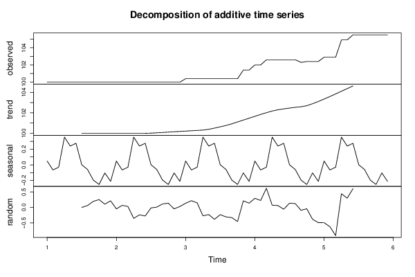
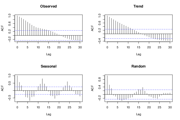
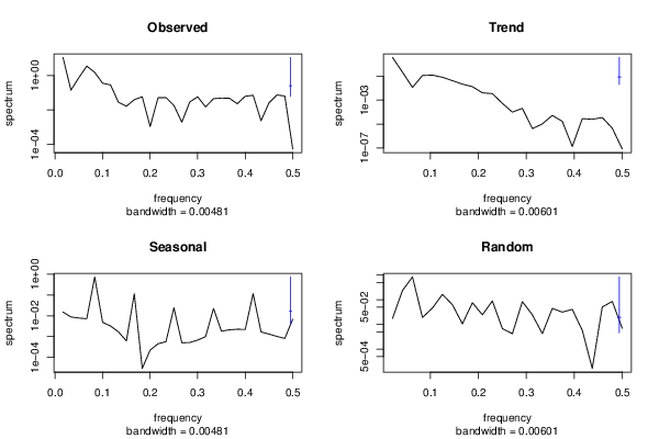
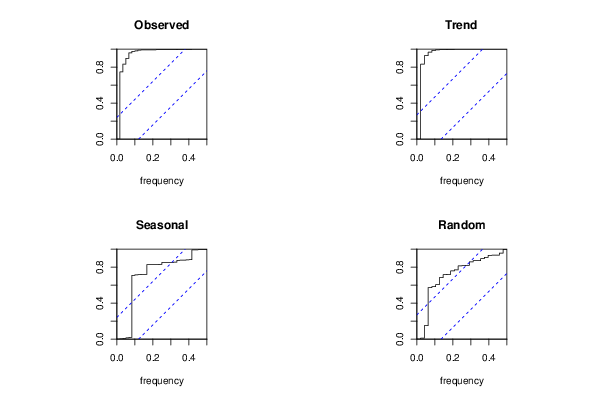
Title produced by software

Classical Decomposition

Date of computation

Sun, 03 Jan 2016 15:52:34 +0000

Cite this page as follows

Statistical Computations at FreeStatistics.org, Office for Research Development and Education, URL https://freestatistics.org/blog/index.php?v=date/2016/Jan/03/t1451836409cj0tcukpiav6n23.htm/, Retrieved Fri, 17 May 2024 04:20:06 +0000

Statistical Computations at FreeStatistics.org, Office for Research Development and Education, URL https://freestatistics.org/blog/index.php?pk=287304, Retrieved Fri, 17 May 2024 04:20:06 +0000

QR Codes:

Paste this QR Code to cite your computation.

Original text written by user:

IsPrivate?

No (this computation is public)

User-defined keywords

Estimated Impact

128

Family? (F = Feedback message, R = changed R code, M = changed R Module, P = changed Parameters, D = changed Data)

-     [Univariate Data Series] [] [2015-09-25 19:44:43] [ba9845715efdcdf5bf90594b26d5ea9c]
- R PD  [Univariate Data Series] [] [2015-10-02 11:08:09] [ba9845715efdcdf5bf90594b26d5ea9c]
- RMP     [Histogram] [] [2015-10-02 11:09:44] [ba9845715efdcdf5bf90594b26d5ea9c]
- RMPD        [Classical Decomposition] [] [2016-01-03 15:52:34] [eed3b94f44ab74d862a61d666a631b56] [Current]

Feedback Forum

Post a new message

Dataseries X:

Download CSV

Histogram

Boxplots

Summary of computational transaction
Raw Input	view raw input (R code)
Raw Output	view raw output of R engine
Computing time	2 seconds
R Server	'Sir Maurice George Kendall' @ kendall.wessa.net

\begin{tabular}{lllllllll}
\hline
Summary of computational transaction \tabularnewline
Raw Input & view raw input (R code)  \tabularnewline
Raw Output & view raw output of R engine  \tabularnewline
Computing time & 2 seconds \tabularnewline
R Server & 'Sir Maurice George Kendall' @ kendall.wessa.net \tabularnewline
\hline
\end{tabular}
%Source: https://freestatistics.org/blog/index.php?pk=287304&T=0

[TABLE]
[ROW][C]Summary of computational transaction[/C][/ROW]
[ROW][C]Raw Input[/C][C]view raw input (R code) [/C][/ROW]
[ROW][C]Raw Output[/C][C]view raw output of R engine [/C][/ROW]
[ROW][C]Computing time[/C][C]2 seconds[/C][/ROW]
[ROW][C]R Server[/C][C]'Sir Maurice George Kendall' @ kendall.wessa.net[/C][/ROW]
[/TABLE]
Source: https://freestatistics.org/blog/index.php?pk=287304&T=0

Globally Unique Identifier (entire table): ba.freestatistics.org/blog/index.php?pk=287304&T=0

As an alternative you can also use a QR Code:

The GUIDs for individual cells are displayed in the table below:

Summary of computational transaction
Raw Input	view raw input (R code)
Raw Output	view raw output of R engine
Computing time	2 seconds
R Server	'Sir Maurice George Kendall' @ kendall.wessa.net

Classical Decomposition by Moving Averages
t	Observations	Fit	Trend	Seasonal	Random
1	100	NA	NA	0.0484375	NA
2	100	NA	NA	-0.0661458	NA
3	100	NA	NA	-0.0307292	NA
4	100	NA	NA	0.354687	NA
5	100	NA	NA	0.240104	NA
6	100	NA	NA	0.275521	NA
7	100	100.001	100	0.000520833	-0.000520833
8	100	99.9401	100	-0.0598958	0.0598958
9	100	99.8047	100	-0.195312	0.195313
10	100	99.7484	100	-0.251562	0.251563
11	100	99.8964	100	-0.103646	0.103646
12	100	99.788	100	-0.211979	0.211979
13	100	100.048	100	0.0484375	-0.0484375
14	100	99.9339	100	-0.0661458	0.0661458
15	100	99.9693	100	-0.0307292	0.0307292
16	100	100.355	100	0.354687	-0.354687
17	100	100.24	100	0.240104	-0.240104
18	100	100.276	100	0.275521	-0.275521
19	100	100.017	100.017	0.000520833	-0.0171875
20	100	99.9901	100.05	-0.0598958	0.00989583
21	100	99.888	100.083	-0.195312	0.111979
22	100	99.8651	100.117	-0.251562	0.134896
23	100	100.046	100.15	-0.103646	-0.0463542
24	100	99.9714	100.183	-0.211979	0.0286458
25	100.4	100.265	100.217	0.0484375	0.134896
26	100.4	100.184	100.25	-0.0661458	0.216146
27	100.4	100.253	100.283	-0.0307292	0.147396
28	100.4	100.671	100.317	0.354687	-0.271354
29	100.4	100.632	100.392	0.240104	-0.231771
30	100.4	100.784	100.508	0.275521	-0.383854
31	100.4	100.634	100.633	0.000520833	-0.233854
32	100.4	100.707	100.767	-0.0598958	-0.306771
33	100.4	100.73	100.925	-0.195312	-0.329688
34	100.4	100.857	101.108	-0.251562	-0.456771
35	101.4	101.188	101.292	-0.103646	0.211979
36	101.4	101.263	101.475	-0.211979	0.136979
37	102	101.707	101.658	0.0484375	0.293229
38	102	101.776	101.842	-0.0661458	0.224479
39	102.6	101.982	102.012	-0.0307292	0.618229
40	102.6	102.53	102.175	0.354687	0.0703125
41	102.6	102.54	102.3	0.240104	0.0598958
42	102.6	102.659	102.383	0.275521	-0.0588542
43	102.6	102.463	102.462	0.000520833	0.136979
44	102.6	102.478	102.537	-0.0598958	0.122396
45	102.3	102.392	102.587	-0.195312	-0.0921875
46	102.4	102.444	102.696	-0.251562	-0.0442708
47	102.4	102.784	102.888	-0.103646	-0.383854
48	102.4	102.892	103.104	-0.211979	-0.492187
49	102.9	103.394	103.346	0.0484375	-0.494271
50	102.9	103.521	103.588	-0.0661458	-0.621354
51	102.9	103.811	103.842	-0.0307292	-0.910938
52	104.9	104.459	104.104	0.354687	0.441146
53	104.9	104.603	104.362	0.240104	0.297396
54	105.5	104.896	104.621	0.275521	0.603646
55	105.5	NA	NA	0.000520833	NA
56	105.5	NA	NA	-0.0598958	NA
57	105.5	NA	NA	-0.195312	NA
58	105.5	NA	NA	-0.251562	NA
59	105.5	NA	NA	-0.103646	NA
60	105.5	NA	NA	-0.211979	NA

\begin{tabular}{lllllllll}
\hline
Classical Decomposition by Moving Averages \tabularnewline
t & Observations & Fit & Trend & Seasonal & Random \tabularnewline
1 & 100 & NA & NA & 0.0484375 & NA \tabularnewline
2 & 100 & NA & NA & -0.0661458 & NA \tabularnewline
3 & 100 & NA & NA & -0.0307292 & NA \tabularnewline
4 & 100 & NA & NA & 0.354687 & NA \tabularnewline
5 & 100 & NA & NA & 0.240104 & NA \tabularnewline
6 & 100 & NA & NA & 0.275521 & NA \tabularnewline
7 & 100 & 100.001 & 100 & 0.000520833 & -0.000520833 \tabularnewline
8 & 100 & 99.9401 & 100 & -0.0598958 & 0.0598958 \tabularnewline
9 & 100 & 99.8047 & 100 & -0.195312 & 0.195313 \tabularnewline
10 & 100 & 99.7484 & 100 & -0.251562 & 0.251563 \tabularnewline
11 & 100 & 99.8964 & 100 & -0.103646 & 0.103646 \tabularnewline
12 & 100 & 99.788 & 100 & -0.211979 & 0.211979 \tabularnewline
13 & 100 & 100.048 & 100 & 0.0484375 & -0.0484375 \tabularnewline
14 & 100 & 99.9339 & 100 & -0.0661458 & 0.0661458 \tabularnewline
15 & 100 & 99.9693 & 100 & -0.0307292 & 0.0307292 \tabularnewline
16 & 100 & 100.355 & 100 & 0.354687 & -0.354687 \tabularnewline
17 & 100 & 100.24 & 100 & 0.240104 & -0.240104 \tabularnewline
18 & 100 & 100.276 & 100 & 0.275521 & -0.275521 \tabularnewline
19 & 100 & 100.017 & 100.017 & 0.000520833 & -0.0171875 \tabularnewline
20 & 100 & 99.9901 & 100.05 & -0.0598958 & 0.00989583 \tabularnewline
21 & 100 & 99.888 & 100.083 & -0.195312 & 0.111979 \tabularnewline
22 & 100 & 99.8651 & 100.117 & -0.251562 & 0.134896 \tabularnewline
23 & 100 & 100.046 & 100.15 & -0.103646 & -0.0463542 \tabularnewline
24 & 100 & 99.9714 & 100.183 & -0.211979 & 0.0286458 \tabularnewline
25 & 100.4 & 100.265 & 100.217 & 0.0484375 & 0.134896 \tabularnewline
26 & 100.4 & 100.184 & 100.25 & -0.0661458 & 0.216146 \tabularnewline
27 & 100.4 & 100.253 & 100.283 & -0.0307292 & 0.147396 \tabularnewline
28 & 100.4 & 100.671 & 100.317 & 0.354687 & -0.271354 \tabularnewline
29 & 100.4 & 100.632 & 100.392 & 0.240104 & -0.231771 \tabularnewline
30 & 100.4 & 100.784 & 100.508 & 0.275521 & -0.383854 \tabularnewline
31 & 100.4 & 100.634 & 100.633 & 0.000520833 & -0.233854 \tabularnewline
32 & 100.4 & 100.707 & 100.767 & -0.0598958 & -0.306771 \tabularnewline
33 & 100.4 & 100.73 & 100.925 & -0.195312 & -0.329688 \tabularnewline
34 & 100.4 & 100.857 & 101.108 & -0.251562 & -0.456771 \tabularnewline
35 & 101.4 & 101.188 & 101.292 & -0.103646 & 0.211979 \tabularnewline
36 & 101.4 & 101.263 & 101.475 & -0.211979 & 0.136979 \tabularnewline
37 & 102 & 101.707 & 101.658 & 0.0484375 & 0.293229 \tabularnewline
38 & 102 & 101.776 & 101.842 & -0.0661458 & 0.224479 \tabularnewline
39 & 102.6 & 101.982 & 102.012 & -0.0307292 & 0.618229 \tabularnewline
40 & 102.6 & 102.53 & 102.175 & 0.354687 & 0.0703125 \tabularnewline
41 & 102.6 & 102.54 & 102.3 & 0.240104 & 0.0598958 \tabularnewline
42 & 102.6 & 102.659 & 102.383 & 0.275521 & -0.0588542 \tabularnewline
43 & 102.6 & 102.463 & 102.462 & 0.000520833 & 0.136979 \tabularnewline
44 & 102.6 & 102.478 & 102.537 & -0.0598958 & 0.122396 \tabularnewline
45 & 102.3 & 102.392 & 102.587 & -0.195312 & -0.0921875 \tabularnewline
46 & 102.4 & 102.444 & 102.696 & -0.251562 & -0.0442708 \tabularnewline
47 & 102.4 & 102.784 & 102.888 & -0.103646 & -0.383854 \tabularnewline
48 & 102.4 & 102.892 & 103.104 & -0.211979 & -0.492187 \tabularnewline
49 & 102.9 & 103.394 & 103.346 & 0.0484375 & -0.494271 \tabularnewline
50 & 102.9 & 103.521 & 103.588 & -0.0661458 & -0.621354 \tabularnewline
51 & 102.9 & 103.811 & 103.842 & -0.0307292 & -0.910938 \tabularnewline
52 & 104.9 & 104.459 & 104.104 & 0.354687 & 0.441146 \tabularnewline
53 & 104.9 & 104.603 & 104.362 & 0.240104 & 0.297396 \tabularnewline
54 & 105.5 & 104.896 & 104.621 & 0.275521 & 0.603646 \tabularnewline
55 & 105.5 & NA & NA & 0.000520833 & NA \tabularnewline
56 & 105.5 & NA & NA & -0.0598958 & NA \tabularnewline
57 & 105.5 & NA & NA & -0.195312 & NA \tabularnewline
58 & 105.5 & NA & NA & -0.251562 & NA \tabularnewline
59 & 105.5 & NA & NA & -0.103646 & NA \tabularnewline
60 & 105.5 & NA & NA & -0.211979 & NA \tabularnewline
\hline
\end{tabular}
%Source: https://freestatistics.org/blog/index.php?pk=287304&T=1

[TABLE]
[ROW][C]Classical Decomposition by Moving Averages[/C][/ROW]
[ROW][C]t[/C][C]Observations[/C][C]Fit[/C][C]Trend[/C][C]Seasonal[/C][C]Random[/C][/ROW]
[ROW][C]1[/C][C]100[/C][C]NA[/C][C]NA[/C][C]0.0484375[/C][C]NA[/C][/ROW]
[ROW][C]2[/C][C]100[/C][C]NA[/C][C]NA[/C][C]-0.0661458[/C][C]NA[/C][/ROW]
[ROW][C]3[/C][C]100[/C][C]NA[/C][C]NA[/C][C]-0.0307292[/C][C]NA[/C][/ROW]
[ROW][C]4[/C][C]100[/C][C]NA[/C][C]NA[/C][C]0.354687[/C][C]NA[/C][/ROW]
[ROW][C]5[/C][C]100[/C][C]NA[/C][C]NA[/C][C]0.240104[/C][C]NA[/C][/ROW]
[ROW][C]6[/C][C]100[/C][C]NA[/C][C]NA[/C][C]0.275521[/C][C]NA[/C][/ROW]
[ROW][C]7[/C][C]100[/C][C]100.001[/C][C]100[/C][C]0.000520833[/C][C]-0.000520833[/C][/ROW]
[ROW][C]8[/C][C]100[/C][C]99.9401[/C][C]100[/C][C]-0.0598958[/C][C]0.0598958[/C][/ROW]
[ROW][C]9[/C][C]100[/C][C]99.8047[/C][C]100[/C][C]-0.195312[/C][C]0.195313[/C][/ROW]
[ROW][C]10[/C][C]100[/C][C]99.7484[/C][C]100[/C][C]-0.251562[/C][C]0.251563[/C][/ROW]
[ROW][C]11[/C][C]100[/C][C]99.8964[/C][C]100[/C][C]-0.103646[/C][C]0.103646[/C][/ROW]
[ROW][C]12[/C][C]100[/C][C]99.788[/C][C]100[/C][C]-0.211979[/C][C]0.211979[/C][/ROW]
[ROW][C]13[/C][C]100[/C][C]100.048[/C][C]100[/C][C]0.0484375[/C][C]-0.0484375[/C][/ROW]
[ROW][C]14[/C][C]100[/C][C]99.9339[/C][C]100[/C][C]-0.0661458[/C][C]0.0661458[/C][/ROW]
[ROW][C]15[/C][C]100[/C][C]99.9693[/C][C]100[/C][C]-0.0307292[/C][C]0.0307292[/C][/ROW]
[ROW][C]16[/C][C]100[/C][C]100.355[/C][C]100[/C][C]0.354687[/C][C]-0.354687[/C][/ROW]
[ROW][C]17[/C][C]100[/C][C]100.24[/C][C]100[/C][C]0.240104[/C][C]-0.240104[/C][/ROW]
[ROW][C]18[/C][C]100[/C][C]100.276[/C][C]100[/C][C]0.275521[/C][C]-0.275521[/C][/ROW]
[ROW][C]19[/C][C]100[/C][C]100.017[/C][C]100.017[/C][C]0.000520833[/C][C]-0.0171875[/C][/ROW]
[ROW][C]20[/C][C]100[/C][C]99.9901[/C][C]100.05[/C][C]-0.0598958[/C][C]0.00989583[/C][/ROW]
[ROW][C]21[/C][C]100[/C][C]99.888[/C][C]100.083[/C][C]-0.195312[/C][C]0.111979[/C][/ROW]
[ROW][C]22[/C][C]100[/C][C]99.8651[/C][C]100.117[/C][C]-0.251562[/C][C]0.134896[/C][/ROW]
[ROW][C]23[/C][C]100[/C][C]100.046[/C][C]100.15[/C][C]-0.103646[/C][C]-0.0463542[/C][/ROW]
[ROW][C]24[/C][C]100[/C][C]99.9714[/C][C]100.183[/C][C]-0.211979[/C][C]0.0286458[/C][/ROW]
[ROW][C]25[/C][C]100.4[/C][C]100.265[/C][C]100.217[/C][C]0.0484375[/C][C]0.134896[/C][/ROW]
[ROW][C]26[/C][C]100.4[/C][C]100.184[/C][C]100.25[/C][C]-0.0661458[/C][C]0.216146[/C][/ROW]
[ROW][C]27[/C][C]100.4[/C][C]100.253[/C][C]100.283[/C][C]-0.0307292[/C][C]0.147396[/C][/ROW]
[ROW][C]28[/C][C]100.4[/C][C]100.671[/C][C]100.317[/C][C]0.354687[/C][C]-0.271354[/C][/ROW]
[ROW][C]29[/C][C]100.4[/C][C]100.632[/C][C]100.392[/C][C]0.240104[/C][C]-0.231771[/C][/ROW]
[ROW][C]30[/C][C]100.4[/C][C]100.784[/C][C]100.508[/C][C]0.275521[/C][C]-0.383854[/C][/ROW]
[ROW][C]31[/C][C]100.4[/C][C]100.634[/C][C]100.633[/C][C]0.000520833[/C][C]-0.233854[/C][/ROW]
[ROW][C]32[/C][C]100.4[/C][C]100.707[/C][C]100.767[/C][C]-0.0598958[/C][C]-0.306771[/C][/ROW]
[ROW][C]33[/C][C]100.4[/C][C]100.73[/C][C]100.925[/C][C]-0.195312[/C][C]-0.329688[/C][/ROW]
[ROW][C]34[/C][C]100.4[/C][C]100.857[/C][C]101.108[/C][C]-0.251562[/C][C]-0.456771[/C][/ROW]
[ROW][C]35[/C][C]101.4[/C][C]101.188[/C][C]101.292[/C][C]-0.103646[/C][C]0.211979[/C][/ROW]
[ROW][C]36[/C][C]101.4[/C][C]101.263[/C][C]101.475[/C][C]-0.211979[/C][C]0.136979[/C][/ROW]
[ROW][C]37[/C][C]102[/C][C]101.707[/C][C]101.658[/C][C]0.0484375[/C][C]0.293229[/C][/ROW]
[ROW][C]38[/C][C]102[/C][C]101.776[/C][C]101.842[/C][C]-0.0661458[/C][C]0.224479[/C][/ROW]
[ROW][C]39[/C][C]102.6[/C][C]101.982[/C][C]102.012[/C][C]-0.0307292[/C][C]0.618229[/C][/ROW]
[ROW][C]40[/C][C]102.6[/C][C]102.53[/C][C]102.175[/C][C]0.354687[/C][C]0.0703125[/C][/ROW]
[ROW][C]41[/C][C]102.6[/C][C]102.54[/C][C]102.3[/C][C]0.240104[/C][C]0.0598958[/C][/ROW]
[ROW][C]42[/C][C]102.6[/C][C]102.659[/C][C]102.383[/C][C]0.275521[/C][C]-0.0588542[/C][/ROW]
[ROW][C]43[/C][C]102.6[/C][C]102.463[/C][C]102.462[/C][C]0.000520833[/C][C]0.136979[/C][/ROW]
[ROW][C]44[/C][C]102.6[/C][C]102.478[/C][C]102.537[/C][C]-0.0598958[/C][C]0.122396[/C][/ROW]
[ROW][C]45[/C][C]102.3[/C][C]102.392[/C][C]102.587[/C][C]-0.195312[/C][C]-0.0921875[/C][/ROW]
[ROW][C]46[/C][C]102.4[/C][C]102.444[/C][C]102.696[/C][C]-0.251562[/C][C]-0.0442708[/C][/ROW]
[ROW][C]47[/C][C]102.4[/C][C]102.784[/C][C]102.888[/C][C]-0.103646[/C][C]-0.383854[/C][/ROW]
[ROW][C]48[/C][C]102.4[/C][C]102.892[/C][C]103.104[/C][C]-0.211979[/C][C]-0.492187[/C][/ROW]
[ROW][C]49[/C][C]102.9[/C][C]103.394[/C][C]103.346[/C][C]0.0484375[/C][C]-0.494271[/C][/ROW]
[ROW][C]50[/C][C]102.9[/C][C]103.521[/C][C]103.588[/C][C]-0.0661458[/C][C]-0.621354[/C][/ROW]
[ROW][C]51[/C][C]102.9[/C][C]103.811[/C][C]103.842[/C][C]-0.0307292[/C][C]-0.910938[/C][/ROW]
[ROW][C]52[/C][C]104.9[/C][C]104.459[/C][C]104.104[/C][C]0.354687[/C][C]0.441146[/C][/ROW]
[ROW][C]53[/C][C]104.9[/C][C]104.603[/C][C]104.362[/C][C]0.240104[/C][C]0.297396[/C][/ROW]
[ROW][C]54[/C][C]105.5[/C][C]104.896[/C][C]104.621[/C][C]0.275521[/C][C]0.603646[/C][/ROW]
[ROW][C]55[/C][C]105.5[/C][C]NA[/C][C]NA[/C][C]0.000520833[/C][C]NA[/C][/ROW]
[ROW][C]56[/C][C]105.5[/C][C]NA[/C][C]NA[/C][C]-0.0598958[/C][C]NA[/C][/ROW]
[ROW][C]57[/C][C]105.5[/C][C]NA[/C][C]NA[/C][C]-0.195312[/C][C]NA[/C][/ROW]
[ROW][C]58[/C][C]105.5[/C][C]NA[/C][C]NA[/C][C]-0.251562[/C][C]NA[/C][/ROW]
[ROW][C]59[/C][C]105.5[/C][C]NA[/C][C]NA[/C][C]-0.103646[/C][C]NA[/C][/ROW]
[ROW][C]60[/C][C]105.5[/C][C]NA[/C][C]NA[/C][C]-0.211979[/C][C]NA[/C][/ROW]
[/TABLE]
Source: https://freestatistics.org/blog/index.php?pk=287304&T=1

Globally Unique Identifier (entire table): ba.freestatistics.org/blog/index.php?pk=287304&T=1

As an alternative you can also use a QR Code:

The GUIDs for individual cells are displayed in the table below:

Classical Decomposition by Moving Averages
t	Observations	Fit	Trend	Seasonal	Random
1	100	NA	NA	0.0484375	NA
2	100	NA	NA	-0.0661458	NA
3	100	NA	NA	-0.0307292	NA
4	100	NA	NA	0.354687	NA
5	100	NA	NA	0.240104	NA
6	100	NA	NA	0.275521	NA
7	100	100.001	100	0.000520833	-0.000520833
8	100	99.9401	100	-0.0598958	0.0598958
9	100	99.8047	100	-0.195312	0.195313
10	100	99.7484	100	-0.251562	0.251563
11	100	99.8964	100	-0.103646	0.103646
12	100	99.788	100	-0.211979	0.211979
13	100	100.048	100	0.0484375	-0.0484375
14	100	99.9339	100	-0.0661458	0.0661458
15	100	99.9693	100	-0.0307292	0.0307292
16	100	100.355	100	0.354687	-0.354687
17	100	100.24	100	0.240104	-0.240104
18	100	100.276	100	0.275521	-0.275521
19	100	100.017	100.017	0.000520833	-0.0171875
20	100	99.9901	100.05	-0.0598958	0.00989583
21	100	99.888	100.083	-0.195312	0.111979
22	100	99.8651	100.117	-0.251562	0.134896
23	100	100.046	100.15	-0.103646	-0.0463542
24	100	99.9714	100.183	-0.211979	0.0286458
25	100.4	100.265	100.217	0.0484375	0.134896
26	100.4	100.184	100.25	-0.0661458	0.216146
27	100.4	100.253	100.283	-0.0307292	0.147396
28	100.4	100.671	100.317	0.354687	-0.271354
29	100.4	100.632	100.392	0.240104	-0.231771
30	100.4	100.784	100.508	0.275521	-0.383854
31	100.4	100.634	100.633	0.000520833	-0.233854
32	100.4	100.707	100.767	-0.0598958	-0.306771
33	100.4	100.73	100.925	-0.195312	-0.329688
34	100.4	100.857	101.108	-0.251562	-0.456771
35	101.4	101.188	101.292	-0.103646	0.211979
36	101.4	101.263	101.475	-0.211979	0.136979
37	102	101.707	101.658	0.0484375	0.293229
38	102	101.776	101.842	-0.0661458	0.224479
39	102.6	101.982	102.012	-0.0307292	0.618229
40	102.6	102.53	102.175	0.354687	0.0703125
41	102.6	102.54	102.3	0.240104	0.0598958
42	102.6	102.659	102.383	0.275521	-0.0588542
43	102.6	102.463	102.462	0.000520833	0.136979
44	102.6	102.478	102.537	-0.0598958	0.122396
45	102.3	102.392	102.587	-0.195312	-0.0921875
46	102.4	102.444	102.696	-0.251562	-0.0442708
47	102.4	102.784	102.888	-0.103646	-0.383854
48	102.4	102.892	103.104	-0.211979	-0.492187
49	102.9	103.394	103.346	0.0484375	-0.494271
50	102.9	103.521	103.588	-0.0661458	-0.621354
51	102.9	103.811	103.842	-0.0307292	-0.910938
52	104.9	104.459	104.104	0.354687	0.441146
53	104.9	104.603	104.362	0.240104	0.297396
54	105.5	104.896	104.621	0.275521	0.603646
55	105.5	NA	NA	0.000520833	NA
56	105.5	NA	NA	-0.0598958	NA
57	105.5	NA	NA	-0.195312	NA
58	105.5	NA	NA	-0.251562	NA
59	105.5	NA	NA	-0.103646	NA
60	105.5	NA	NA	-0.211979	NA

Figure 1

PNG link

Postscript link

PDF link

Figure 2

PNG link

Postscript link

PDF link

Figure 3

PNG link

Postscript link

PDF link

Figure 4

PNG link

Postscript link

PDF link

Parameters (Session):

par1 = 48 ; par2 = 1 ; par3 = 0 ; par4 = 0 ; par5 = 12 ; par6 = White Noise ; par7 = 0.95 ;

Parameters (R input):

par1 = additive ; par2 = 12 ;

R code (references can be found in the software module):

par2 <- as.numeric(par2)
x <- ts(x,freq=par2)
m <- decompose(x,type=par1)
m$figure
bitmap(file='test1.png')
plot(m)
dev.off()
mylagmax <- length(x)/2
bitmap(file='test2.png')
op <- par(mfrow = c(2,2))
acf(as.numeric(x),lag.max = mylagmax,main='Observed')
acf(as.numeric(m$trend),na.action=na.pass,lag.max = mylagmax,main='Trend')
acf(as.numeric(m$seasonal),na.action=na.pass,lag.max = mylagmax,main='Seasonal')
acf(as.numeric(m$random),na.action=na.pass,lag.max = mylagmax,main='Random')
par(op)
dev.off()
bitmap(file='test3.png')
op <- par(mfrow = c(2,2))
spectrum(as.numeric(x),main='Observed')
spectrum(as.numeric(m$trend[!is.na(m$trend)]),main='Trend')
spectrum(as.numeric(m$seasonal[!is.na(m$seasonal)]),main='Seasonal')
spectrum(as.numeric(m$random[!is.na(m$random)]),main='Random')
par(op)
dev.off()
bitmap(file='test4.png')
op <- par(mfrow = c(2,2))
cpgram(as.numeric(x),main='Observed')
cpgram(as.numeric(m$trend[!is.na(m$trend)]),main='Trend')
cpgram(as.numeric(m$seasonal[!is.na(m$seasonal)]),main='Seasonal')
cpgram(as.numeric(m$random[!is.na(m$random)]),main='Random')
par(op)
dev.off()
load(file='createtable')
a<-table.start()
a<-table.row.start(a)
a<-table.element(a,'Classical Decomposition by Moving Averages',6,TRUE)
a<-table.row.end(a)
a<-table.row.start(a)
a<-table.element(a,'t',header=TRUE)
a<-table.element(a,'Observations',header=TRUE)
a<-table.element(a,'Fit',header=TRUE)
a<-table.element(a,'Trend',header=TRUE)
a<-table.element(a,'Seasonal',header=TRUE)
a<-table.element(a,'Random',header=TRUE)
a<-table.row.end(a)
for (i in 1:length(m$trend)) {
a<-table.row.start(a)
a<-table.element(a,i,header=TRUE)
a<-table.element(a,x[i])
if (par1 == 'additive') a<-table.element(a,signif(m$trend[i]+m$seasonal[i],6)) else a<-table.element(a,signif(m$trend[i]*m$seasonal[i],6))
a<-table.element(a,signif(m$trend[i],6))
a<-table.element(a,signif(m$seasonal[i],6))
a<-table.element(a,signif(m$random[i],6))
a<-table.row.end(a)
}
a<-table.end(a)
table.save(a,file='mytable.tab')

Free Statistics

Description of Statistical Computation

Tree of Dependent Computations

Dataset

Tables (Output of Computation)

Figures (Output of Computation)

Input Parameters & R Code