Free Statistics
of Irreproducible Research!
Description of Statistical Computation | |||||||||||||||||||||
|---|---|---|---|---|---|---|---|---|---|---|---|---|---|---|---|---|---|---|---|---|---|
| Author's title | |||||||||||||||||||||
| Author | *Unverified author* | ||||||||||||||||||||
| R Software Module | rwasp_meanplot.wasp | ||||||||||||||||||||
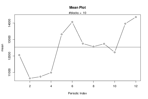
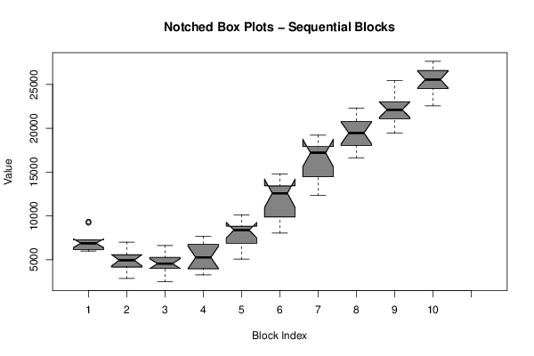
| Title produced by software | Mean Plot | ||||||||||||||||||||
| Date of computation | Tue, 09 Aug 2016 13:21:50 +0100 | ||||||||||||||||||||
| Cite this page as follows | Statistical Computations at FreeStatistics.org, Office for Research Development and Education, URL https://freestatistics.org/blog/index.php?v=date/2016/Aug/09/t14707453373gbk5o0i19hc9hs.htm/, Retrieved Sat, 18 May 2024 16:43:23 +0000 | ||||||||||||||||||||
| Statistical Computations at FreeStatistics.org, Office for Research Development and Education, URL https://freestatistics.org/blog/index.php?pk=296141, Retrieved Sat, 18 May 2024 16:43:23 +0000 | |||||||||||||||||||||
| QR Codes: | |||||||||||||||||||||
|
| |||||||||||||||||||||
| Original text written by user: | |||||||||||||||||||||
| IsPrivate? | No (this computation is public) | ||||||||||||||||||||
| User-defined keywords | |||||||||||||||||||||
| Estimated Impact | 130 | ||||||||||||||||||||
Tree of Dependent Computations | |||||||||||||||||||||
| Family? (F = Feedback message, R = changed R code, M = changed R Module, P = changed Parameters, D = changed Data) | |||||||||||||||||||||
| - [Univariate Data Series] [] [2016-08-09 07:18:36] [ba9845715efdcdf5bf90594b26d5ea9c] - PD [Univariate Data Series] [] [2016-08-09 07:23:22] [ba9845715efdcdf5bf90594b26d5ea9c] - RMPD [Mean Plot] [] [2016-08-09 12:21:50] [eed3b94f44ab74d862a61d666a631b56] [Current] | |||||||||||||||||||||
| Feedback Forum | |||||||||||||||||||||
Post a new message | |||||||||||||||||||||
Dataset | |||||||||||||||||||||
| Dataseries X: | |||||||||||||||||||||
7263.63 7135.88 7008.00 6752.38 9339.00 9211.13 7263.63 5970.38 6098.13 6098.13 6226.00 6495.50 5714.75 4932.75 4292.38 4292.38 6752.38 7008.00 5060.50 2857.38 4022.88 4022.88 4932.75 5457.88 5330.00 4022.88 4677.13 4420.25 6623.38 6098.13 4022.88 2472.75 3895.00 4292.38 4677.13 5188.38 4150.63 3254.75 3639.50 3767.25 7135.88 7135.88 5188.38 4932.75 5714.75 5330.00 6367.75 7661.00 7917.88 6098.13 5585.63 5060.50 8570.88 8827.75 8173.50 8827.75 8698.63 7661.00 8827.75 10121.00 10646.13 9083.38 8045.63 8827.75 12196.25 13234.00 12978.38 13489.50 13361.75 12068.50 14271.63 14796.75 15564.88 13234.00 12324.13 13361.75 15834.38 18037.50 17512.38 17512.38 17769.25 16872.00 19204.25 19204.25 18806.88 16602.50 16999.88 17256.75 18947.38 21150.50 19587.63 20369.75 19715.50 19332.00 22317.25 21663.00 20753.13 19459.88 20753.13 21407.38 22188.13 23225.75 22188.13 22828.50 22047.63 21919.88 25160.63 25430.13 24392.50 22572.88 24123.00 24776.00 25558.00 26723.50 25558.00 26467.88 26070.50 24648.13 27633.25 27633.25 | |||||||||||||||||||||
Tables (Output of Computation) | |||||||||||||||||||||
| |||||||||||||||||||||
Figures (Output of Computation) | |||||||||||||||||||||
Input Parameters & R Code | |||||||||||||||||||||
| Parameters (Session): | |||||||||||||||||||||
| par1 = grey ; par2 = no ; | |||||||||||||||||||||
| Parameters (R input): | |||||||||||||||||||||
| par1 = 12 ; | |||||||||||||||||||||
| R code (references can be found in the software module): | |||||||||||||||||||||
par1 <- as.numeric(par1) | |||||||||||||||||||||