Free Statistics
of Irreproducible Research!
Description of Statistical Computation | |||||||||||||||||||||
|---|---|---|---|---|---|---|---|---|---|---|---|---|---|---|---|---|---|---|---|---|---|
| Author's title | |||||||||||||||||||||
| Author | *Unverified author* | ||||||||||||||||||||
| R Software Module | rwasp_meanplot.wasp | ||||||||||||||||||||
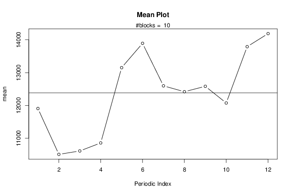
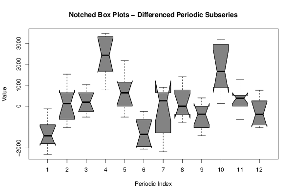
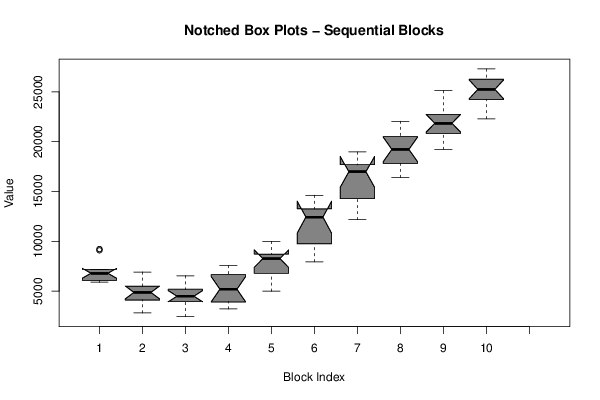
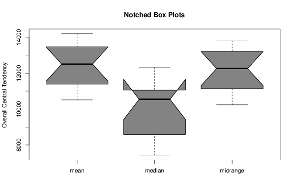
| Title produced by software | Mean Plot | ||||||||||||||||||||
| Date of computation | Mon, 08 Aug 2016 15:57:53 +0100 | ||||||||||||||||||||
| Cite this page as follows | Statistical Computations at FreeStatistics.org, Office for Research Development and Education, URL https://freestatistics.org/blog/index.php?v=date/2016/Aug/08/t14706683152rqdvxvbr4kjkpp.htm/, Retrieved Sat, 18 May 2024 16:16:58 +0000 | ||||||||||||||||||||
| Statistical Computations at FreeStatistics.org, Office for Research Development and Education, URL https://freestatistics.org/blog/index.php?pk=296095, Retrieved Sat, 18 May 2024 16:16:58 +0000 | |||||||||||||||||||||
| QR Codes: | |||||||||||||||||||||
|
| |||||||||||||||||||||
| Original text written by user: | |||||||||||||||||||||
| IsPrivate? | No (this computation is public) | ||||||||||||||||||||
| User-defined keywords | |||||||||||||||||||||
| Estimated Impact | 163 | ||||||||||||||||||||
Tree of Dependent Computations | |||||||||||||||||||||
| Family? (F = Feedback message, R = changed R code, M = changed R Module, P = changed Parameters, D = changed Data) | |||||||||||||||||||||
| - [Central Tendency] [Braadoven Omzet -...] [2016-08-08 13:38:20] [74be16979710d4c4e7c6647856088456] - RMP [Mean Plot] [Braadoven Omzet -...] [2016-08-08 14:57:53] [d41d8cd98f00b204e9800998ecf8427e] [Current] | |||||||||||||||||||||
| Feedback Forum | |||||||||||||||||||||
Post a new message | |||||||||||||||||||||
Dataset | |||||||||||||||||||||
| Dataseries X: | |||||||||||||||||||||
7175 7048.75 6922.5 6670 9225 9098.75 7175 5897.5 6023.75 6023.75 6150 6416.25 5645 4872.5 4240 4240 6670 6922.5 4998.75 2822.5 3973.75 3973.75 4872.5 5391.25 5265 3973.75 4620 4366.25 6542.5 6023.75 3973.75 2442.5 3847.5 4240 4620 5125 4100 3215 3595 3721.25 7048.75 7048.75 5125 4872.5 5645 5265 6290 7567.5 7821.25 6023.75 5517.5 4998.75 8466.25 8720 8073.75 8720 8592.5 7567.5 8720 9997.5 10516.25 8972.5 7947.5 8720 12047.5 13072.5 12820 13325 13198.75 11921.25 14097.5 14616.25 15375 13072.5 12173.75 13198.75 15641.25 17817.5 17298.75 17298.75 17552.5 16666.25 18970 18970 18577.5 16400 16792.5 17046.25 18716.25 20892.5 19348.75 20121.25 19475 19096.25 22045 21398.75 20500 19222.5 20500 21146.25 21917.5 22942.5 21917.5 22550 21778.75 21652.5 24853.75 25120 24095 22297.5 23828.75 24473.75 25246.25 26397.5 25246.25 26145 25752.5 24347.5 27296.25 27296.25 | |||||||||||||||||||||
Tables (Output of Computation) | |||||||||||||||||||||
| |||||||||||||||||||||
Figures (Output of Computation) | |||||||||||||||||||||
Input Parameters & R Code | |||||||||||||||||||||
| Parameters (Session): | |||||||||||||||||||||
| par1 = 12 ; | |||||||||||||||||||||
| Parameters (R input): | |||||||||||||||||||||
| par1 = 12 ; | |||||||||||||||||||||
| R code (references can be found in the software module): | |||||||||||||||||||||
par1 <- as.numeric(par1) | |||||||||||||||||||||