Free Statistics
of Irreproducible Research!
Description of Statistical Computation | |||||||||||||||||||||
|---|---|---|---|---|---|---|---|---|---|---|---|---|---|---|---|---|---|---|---|---|---|
| Author's title | |||||||||||||||||||||
| Author | *The author of this computation has been verified* | ||||||||||||||||||||
| R Software Module | rwasp_meanplot.wasp | ||||||||||||||||||||
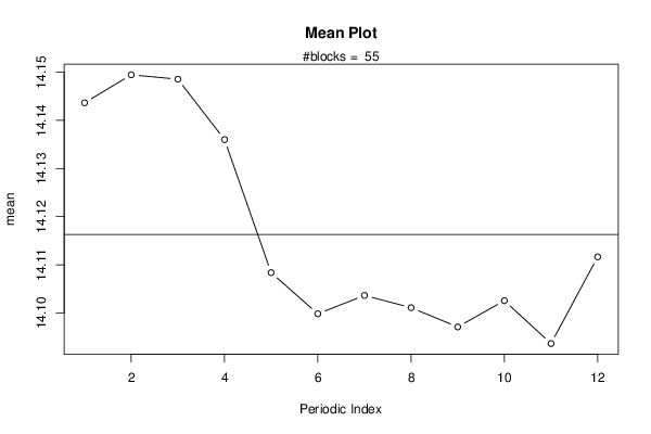
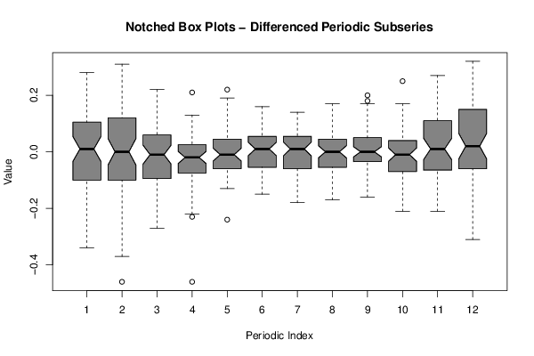
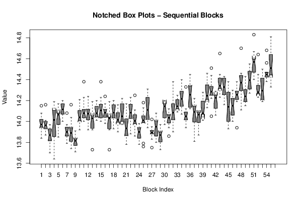
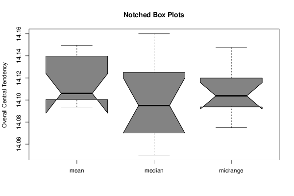
| Title produced by software | Mean Plot | ||||||||||||||||||||
| Date of computation | Tue, 15 Dec 2015 14:44:26 +0000 | ||||||||||||||||||||
| Cite this page as follows | Statistical Computations at FreeStatistics.org, Office for Research Development and Education, URL https://freestatistics.org/blog/index.php?v=date/2015/Dec/15/t1450190682l1pg9n9odgbptqq.htm/, Retrieved Sat, 18 May 2024 15:57:06 +0000 | ||||||||||||||||||||
| Statistical Computations at FreeStatistics.org, Office for Research Development and Education, URL https://freestatistics.org/blog/index.php?pk=286514, Retrieved Sat, 18 May 2024 15:57:06 +0000 | |||||||||||||||||||||
| QR Codes: | |||||||||||||||||||||
|
| |||||||||||||||||||||
| Original text written by user: | |||||||||||||||||||||
| IsPrivate? | No (this computation is public) | ||||||||||||||||||||
| User-defined keywords | |||||||||||||||||||||
| Estimated Impact | 69 | ||||||||||||||||||||
Tree of Dependent Computations | |||||||||||||||||||||
| Family? (F = Feedback message, R = changed R code, M = changed R Module, P = changed Parameters, D = changed Data) | |||||||||||||||||||||
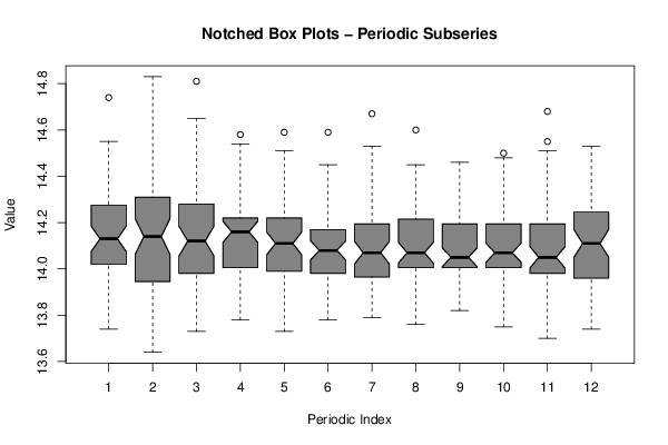
| - [Mean Plot] [Notched Box Plots...] [2015-12-15 14:44:26] [6c9172abf40f1c7e1d0d83ef980264f4] [Current] | |||||||||||||||||||||
| Feedback Forum | |||||||||||||||||||||
Post a new message | |||||||||||||||||||||
Dataset | |||||||||||||||||||||
| Dataseries X: | |||||||||||||||||||||
14.15 13.95 13.96 13.99 14.08 14.03 13.93 13.95 13.94 14.01 13.98 13.84 14.16 13.92 13.97 14 14 13.87 13.94 13.98 13.95 14.01 13.96 13.88 13.76 13.79 13.97 13.84 13.94 13.97 13.92 13.87 13.9 13.85 13.7 13.87 13.74 13.64 13.83 13.88 14.01 13.98 14.02 14.1 14.11 14.14 14.04 14.19 14.17 14.14 13.94 14.09 14.06 14.07 14.07 14.07 14.05 13.99 13.85 13.95 14.13 14.2 14.2 14.18 14.13 14.07 14.06 14.07 14.1 14.1 14 14.16 13.85 13.97 13.91 13.9 13.83 13.9 13.79 13.88 13.94 13.95 14.08 13.87 14.16 13.9 13.74 13.82 13.82 13.88 13.9 14.04 13.92 13.96 13.8 13.74 13.84 13.71 13.78 13.78 13.76 13.81 13.87 13.76 13.82 13.82 13.83 13.91 13.92 14 13.99 14.01 14.09 14.13 14.03 14.1 14.05 14.02 14.11 14.21 14.38 14.23 14.1 14.04 14.12 14 14.11 14.03 14.03 14.04 14.06 14.1 14.11 14.12 14.24 14.17 14.08 14.07 14.09 14.02 14.01 13.98 13.92 14.03 14.01 14.19 13.73 13.92 13.94 14.03 14.04 14.03 14.07 14.04 13.93 14.17 14.06 14.2 14.16 14.11 14.16 14.13 14.01 14.05 14.04 14.1 14.05 14.02 14.11 14.21 14.38 14.23 14.1 14.04 14.12 14 14.11 14.03 14.03 14.04 14.06 14.1 14.11 14.12 14.24 14.17 14.08 14.07 14.09 14.02 14.01 13.98 13.92 14.03 14.01 14.19 13.73 13.92 13.94 14.03 14.04 14.03 14.07 14.04 13.93 14.17 14.06 14.2 14.16 14.11 14.16 14.13 14.01 14.05 14.04 14.03 14.04 13.9 14.09 14.16 14.09 14.08 13.95 14.01 14 13.99 14 14.02 14.06 14.02 13.97 14.19 13.97 13.98 14.03 14.04 14.13 14.22 14.21 14.15 14.17 14.03 14.02 13.91 13.81 13.78 13.83 13.96 13.9 14.1 13.99 13.9 13.88 13.89 14.03 14.19 14.16 14.1 14.03 14.06 14.07 14.11 14.17 14.23 14.11 14.25 14.03 14.07 13.99 14.01 13.98 13.93 14.06 13.98 14 13.86 13.98 13.8 13.8 13.89 13.88 13.78 13.89 13.93 13.95 13.92 13.96 13.91 13.76 13.79 13.99 13.99 13.99 14.04 14.01 14.13 14.01 14.07 14.04 14.18 14.26 14.31 14.26 14.2 14.18 14.14 14.08 14 14.04 14.08 14 13.94 13.83 13.75 13.92 13.91 13.91 13.9 13.95 14.02 13.89 13.89 13.89 13.87 14.03 13.96 14.06 13.98 14.08 13.95 13.95 13.84 13.94 13.88 13.83 13.8 13.92 13.9 13.73 13.87 13.76 13.86 13.9 13.85 13.9 13.75 13.87 13.97 13.97 14.14 14.18 14.17 14.2 14.17 14.15 14.1 14.04 14.01 14.15 14.03 14.04 14.05 14.12 14.09 13.98 13.94 14.04 13.86 14.03 13.99 14.08 14.01 14.04 13.9 14.09 14.04 13.97 14.08 13.99 14.11 14.16 14.18 14.18 14.38 14.18 14.22 14.13 14.2 14.25 14.14 14.15 14.13 14.1 14.09 14.23 14.11 14.4 14.3 14.37 14.24 14.14 14.17 14.19 14.24 14.11 14.07 14.15 14.28 14.03 14.06 13.94 14.05 14.12 14 14.12 13.99 14.04 14.05 14.06 14.33 14.45 14.39 14.39 14.23 14.25 14.15 14.12 14.26 14.28 14.12 14.29 14.12 14.22 14.09 14.17 14.01 14.22 13.98 14.12 14.09 14.11 14.05 13.96 13.81 14.09 13.87 14.1 14.08 14.09 14.08 13.95 14.08 14 14.05 13.98 14.04 14.24 14.28 14.23 14.16 14.11 14.07 14.07 14.08 14.02 14.08 14.01 14.08 14.23 14.39 14.13 14.21 14.21 14.26 14.36 14.18 14.34 14.26 14.22 14.46 14.51 14.32 14.44 14.35 14.3 14.32 14.24 14.27 14.26 14.26 14.05 14.22 14.11 14.25 14.26 14.16 14.07 14.06 14.22 14.24 14.25 14.23 14.14 14.29 14.33 14.34 14.65 14.43 14.32 14.31 14.34 14.28 14.23 14.4 14.45 14.39 14.35 14.43 14.29 14.41 14.31 14.42 14.43 14.3 14.36 14.22 14.16 14.2 14.38 14.37 14.34 14.19 14.22 14.15 14 14.01 13.94 14 13.93 14.13 14.28 14.26 14.3 14.18 14.18 14.1 14.09 14.03 14.02 14.16 14 14.14 14.28 13.94 14.25 14.26 14.22 14.29 14.2 14.19 14.25 14.38 14.37 14.29 14.44 14.7 14.44 14.34 14.11 14.33 14.46 14.37 14.24 14.42 14.37 14.26 14.23 14.43 14.25 14.2 14.21 14.18 14.3 14.32 14.16 14.15 14.28 14.31 14.27 14.31 14.46 14.33 14.31 14.43 14.28 14.36 14.45 14.5 14.55 14.53 14.55 14.83 14.56 14.58 14.59 14.59 14.67 14.6 14.43 14.42 14.4 14.51 14.45 14.64 14.27 14.28 14.23 14.28 14.26 14.27 14.25 14.3 14.32 14.37 14.21 14.49 14.46 14.5 14.3 14.31 14.28 14.37 14.29 14.21 14.21 14.19 14.38 14.4 14.56 14.42 14.47 14.45 14.46 14.45 14.45 14.43 14.68 14.47 14.74 14.75 14.81 14.54 14.51 14.43 14.53 14.43 14.46 14.48 14.51 14.33 | |||||||||||||||||||||
Tables (Output of Computation) | |||||||||||||||||||||
| |||||||||||||||||||||
Figures (Output of Computation) | |||||||||||||||||||||
Input Parameters & R Code | |||||||||||||||||||||
| Parameters (Session): | |||||||||||||||||||||
| par1 = 1 ; par2 = 2 ; par3 = 0,99 ; par4 = two.sided ; par5 = paired ; par6 = 0 ; | |||||||||||||||||||||
| Parameters (R input): | |||||||||||||||||||||
| par1 = 12 ; | |||||||||||||||||||||
| R code (references can be found in the software module): | |||||||||||||||||||||
par1 <- as.numeric(par1) | |||||||||||||||||||||